Multiple lineare Regression und Modellselektion

DS3 - Vom experimentellen Design zur
explorativen Datenanalyse & Data Mining

Saskia Otto & Monika Eberhard

Universität Hamburg, IMF

Wintersemester 2025/2026

Lernziele

Am Ende dieser VL- und Übungseinheit werden Sie

die Unterschiede zwischen einer einfachen und einer multiplen Regression kennen.
wissen, warum und wie auf (Multi-)Kollinearität vorab geprüft werden muss.
weitere Kriterien für die Modellauswahl kennen und im Rahmen einer ‘backward selection’ anwenden können.
wissen, was mit Ockhams Rasiermesser gemeint ist.

Regression mit
≥ 2 Kovariaten

Multiple Regression | Ziel

Identifizierung des Einflusses mehrerer unabhängiger Kovariaten X_p auf die Antwortvariable unter Berücksichtigung der Beziehungen zwischen den Kovariaten.
Vorhersage von Y-Werten aus den Werten mehrerer X-Variablen.
Bestimmung der einflussreichsten Parameter aus mehreren unabhängigen Variablen → empirische Variablenauswahl.

Multiple Regression | Gleichung

Die Grundsätze einer einfachen, bivariaten Regressionsanalyse lassen sich auf zwei oder mehr kontinuierliche Variablen ausweiten:

Faustregel: nicht mehr als 10 erklärende Variablen

Multiple Regression | Neu

Zusätzliche Annahmen / Datenexplorationen
Schätzung der Parameter (Achsenabschnitt \alpha & partielle Regressionskoeffizienten \beta_p)
Signifikanztest
(Multiples) R^2 vs. korrigiertes R^2
Modellauswahl

Zusätzliche Annahmen

Wie bei der einfachen (bivariaten) Regression
- Normalität
- Homogenität
- Unabhängigkeit
- Linearität

NEU
- Anzahl der Kovariaten < Anzahl der Beobachtungen (p < n)
- Keine lineare Beziehung zwischen den Kovariaten (keine Kollinearität / Multikollinearität)

Problem der Kollinearität

Kleine Änderungen in den Daten → extreme Änderungen in den Regressionskoeffizienten
Schätzungen zwischen verschiedenen Stichproben derselben Population können stark voneinander abweichen → hohe Standardfehler der geschätzten Parameter
Schätzungen von \beta’s und Signifikanztests unzuverlässig.

Problem der Kollinearität | Demo

Link zur Shiny-App: teaching-stats/collinearity/

Prüfen auf Kollinearität

Paarweise Korrelation und Streudiagramme
Berechnung des VIF-Werts für jede Kovariate → in R z.B. mit car::vif()

VIF-Wert

VIF_i = \frac{1}{TOL_i} = \frac{1}{1-R_i^2}

R^2 hier aus Modell, welches alle Kovariaten enthält, außer der Kovariate, für die der VIF-Wert berechnet wird.
Faustregel: VIF > 3 ist problematisch (einige sagen VIF>10, hängt auch von der Anzahl an Kovariaten ab)
Wenn Kovariaten einen VIF > 3 haben,
- → die Kovariate mit dem höchsten VIF entfernen (oder nach biologischem Wissen/Interesse entscheiden)
- → die VIFs für die verbleibenden Kovariaten neu berechnen
- → fortfahren, bis alle Kovariaten VIFs < 3 haben.

Weitere Datenexploration

Unabhängigkeit (posteriori)
- Visualisieren Sie im Streudiagramm die Residuen gegen die einzelnen erklärenden Variablen (auch diejenigen, die aus dem endgültigen Modell ausgeschlossen wurden) und suchen Sie nach einem Muster.
Interaktionen (a priori)
- Darstellung von Y gegen X_1, X_2,… in Abhängigkeit von einer anderen Kovariate
- Nützliche Funktion coplot()

Parameterschätzung

Achsenabschnitt (intercept) \alpha
- Wert von Y, wenn alle X-Werte gleich Null sind → weniger wichtig
Partielle Regressionskoeffizienten (slopes) \beta_p (\beta_1, \beta_2,.. )
- Effekt einer Erhöhung von X_p um 1 Einheit, wobei alle anderen Kovariaten oder Prädiktoren (X) konstant bleiben
- Regressionskoeffizienten der Stichprobe (a, b_p) werden mit OLS Methode geschätzt.
- \hat{y}_i = a + b_1 x_{1,i} + b_2 x_{2,i} + ...
  \hat{y}_i = \text{vorhergesagter Y-Wert für jede Kombination von X-Werten}

Signifikanztests | Partielle Koeffizienten

H_0:\beta_p = 0
Getrennte t-Tests für jeden partiellen Regressionskoeffizienten im Modell
Partielle t-Tests verwenden: t_p = \frac{b_p}{s.e.(b_p)}
Vergleich mit t-Verteilung mit N-2 Freiheitsgraden
H_0 verwerfen, wenn p < 0.05

Anpassung des Bestimmtheitsmaß

Lösung: korrigiertes Bestimmtheitsmaß

Modellauswahl

Ausgangssituation

Wir wollen das optimale Modell finden, das die Parameter identifiziert, die die gesammelten Daten am besten erklären.
Aber welches von allen möglichen Modellen passt am besten zu den Daten?

Viele mögliche Modelle
- für p Prädiktoren, # mögliche Modelle = 2^p
- → 6 Prädiktoren, 64 mögliche Modelle
- → 10 Prädiktoren, 1024 mögliche Modelle

Effiziente Suchverfahren erforderlich
Verschiedene Ansätze und unterschiedliche Kriterien für die Auswahl des “besten” Modells
Sparsamkeitsprinzip (principle of parsimony)

Sparsamkeitsprinzip

Oder Ockhams Rasiermesser

Das Prinzip der Parsimonie wird dem englischen Philosophen William von Ockham aus dem frühen 14. Jahrhundert zugeschrieben, der darauf bestand, dass bei einer Reihe gleichwertiger Erklärungen für ein bestimmtes Phänomen die einfachste Erklärung die richtige ist. Sie wird Ockhams Rasiermesser genannt, weil er seine Erklärungen auf das absolute Minimum ‘rasierte’.

Ockhams Rasiermesser besagt, dass wir bei zwei gültigen Annahmen immer die einfachste wählen sollten. Wir sollten die einfachste wählen, weil es wahrscheinlicher ist, dass sie die richtige ist.

Kriterien der Modellauswahl

Hypothesentests (z.B. der F-Test)
Korrigiertes R^2 → je höher desto besser → absolutes Maß
Akaike’s Informationskriterium (AIC) → je niedriger desto besser → relatives Maß
- Faustregel: Wenn der Unterschied zwischen 2 Modellen im AIC ≤ 2 beträgt, sollte das einfachere Modell gewählt werden.
- Berücksichtigt das Maß der Anpassungsgüte und fügt einen so genannten Strafterm für die Anzahl der unabhängigen Parameter im Modell hinzu.

Bayesian Informationskriterium (BIC)
- Gibt der Anzahl an Kovariaten mehr Gewicht
- Empfehlenswert, wenn p > 7

‘All subsets selection’

Vergleich ausgewählter Teilmengen von Modellen und Wahl des optimalen Modells mittels AIC oder BIC.
Kann zu einer großen Anzahl von zu vergleichenden Modellen führen.
Viele Iterationen und zeitaufwändig, wenn p > 5.
Die Anzahl kann jedoch reduziert werden, indem a priori einige Teilmengen auf der Grundlage ökologischer Kenntnisse ausgewählt werden.

‘Stepwise selection’

Untersuchung einer Teilmenge möglicher Modelle auf der Grundlage eines bestimmten Kriteriums.
Sog. ‘forward selection’
Sog. ‘backward selection’:
- Startet mit allen Prädiktoren (volles Modell) und entfernt eine Variable bzw. einen Term nach dem anderen bis R_{adj}^2 sinkt bzw. der AIC steigt.
’stepwise selection’:
- kombiniert vorwärts und rückwärts gerichtete Auswahl

‘Backward selection’ | 1

Wir starten mit allen Variablen und Interaktionen

→ Höchstwahrscheinlich viel zu viele Variablen und Interaktionen im Modell.

‘Backward selection’ | 2

Schrittweises Entfernen

Modell sollte möglichst simpel sein → erst die komplexeren, dann die weniger komplexen Terme entfernen.

‘Backward selection’ | 3

Schrittweises Entfernen

Also erst Entfernen komplexer Interaktionsterme (z.B. 4er- vor 3er-Interaktion).
Einzelne Variablen werden (meistens) erst ganz zum Schluss entfernt.
Solange eine Variable in einer Interaktion auftritt, darf die Variable selbst nicht entfernt werden.

‘Backward selection’ | 4

Schrittweises Entfernen

Es ist durchaus möglich, einzelne Variablen zu entfernen, bevor eine Interaktion entfernt wird → solange diese Variablen nicht Teil der Interaktion sind!

Your turn …

01:00

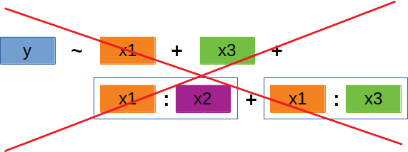
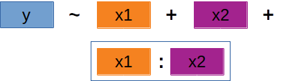
Quiz 1 | Formelschreibweise

Folgender Datensatz ist gegeben:

'data.frame':   20 obs. of  5 variables:
 $ Y : num  508 511 535 534 500 ...
 $ X1: num  4.4 7.7 25.6 10.7 11.3 ...
 $ X2: num  989 998 990 993 994 ...
 $ X3: num  0.244 0.668 0.418 0.788 0.103 ...
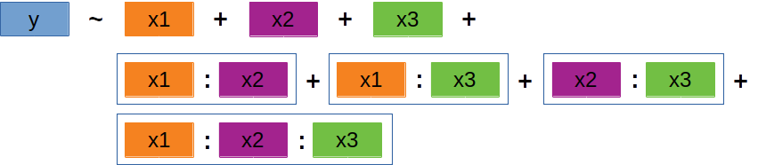
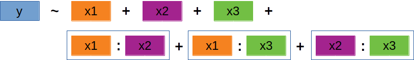
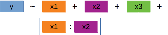
 $ X4: num  3.13 2.99 2.98 3.68 2.89 ...

Erstellen Sie nun die Formel für ein multiples Regressionsmodell, dass die Effekte

der vier Variablen X1, X2, X3, X4,
der 2-Wege Interaktion zwischen X2 und X4,
sowie der 3-Wege-Interaktion zwischen X1, X3, und X4 testet.

Quiz
Erklärung

Höhere Interaktionen messen, wie sich Interaktionseffekte selbst verändern, wenn eine weitere Variable dazu kommt.
Beispiel: der 3-Wege-Term X1:X3:X4 sagt aus, ob die Effekte der 2-Wege-Interaktionen wie X1:X3, X1:X4 und X3:X4 jeweils von der dritten X Variable abhängen.
Damit das interpretierbar ist, braucht man alle drei 2-Wege-Interaktionsterme schon im Modell.

mod <- lm(
  Y ~ X1 + X2 + X3 + X4 + X2:X4 + X1:X3 + X1:X4 + X3:X4 + X1:X3:X4,
  ## alternative Schreibweise:
  # Y ~ X1*X3*X4 + X2 + X2:X4,
  data = df
)

Bei der Modellauswahl dürfen immer nur die höheren Interaktionsterme entfernt werden.
Die zugehörigen niedrigeren Terme (Haupteffekte und 2-Wege-Interaktionen) müssen im Modell bleiben, solange ein höherer Interaktionsterm sie enthält.
In unserem Beispiel könnten also nur die 3-Wege-Terme X1:X3:X4 oder X2:X4 entfernt werden – nicht aber die 2-Wege-Interaktionen, die darin verschachtelt sind.
Genau das berücksichtigt die step()-Funktion automatisch (siehe erster Step; mehr zur Funktion im Praxisbeispiel in R):

step(mod)

Start:  AIC=98.15
Y ~ X1 + X2 + X3 + X4 + X2:X4 + X1:X3 + X1:X4 + X3:X4 + X1:X3:X4

           Df Sum of Sq     RSS    AIC
- X1:X3:X4  1    3.3703  998.99 96.220
- X2:X4     1    9.6507 1005.27 96.346
<none>                   995.62 98.153

Step:  AIC=96.22
Y ~ X1 + X2 + X3 + X4 + X2:X4 + X1:X3 + X1:X4 + X3:X4

        Df Sum of Sq     RSS    AIC
- X3:X4  1     0.377  999.37 94.228
- X2:X4  1     6.806 1005.80 94.356
- X1:X4  1     9.490 1008.48 94.409
<none>                998.99 96.220
- X1:X3  1   114.064 1113.06 96.383

Step:  AIC=94.23
Y ~ X1 + X2 + X3 + X4 + X2:X4 + X1:X3 + X1:X4

        Df Sum of Sq     RSS    AIC
- X2:X4  1     9.225 1008.59 92.412
- X1:X4  1    12.484 1011.85 92.476
<none>                999.37 94.228
- X1:X3  1   124.140 1123.51 94.570

Step:  AIC=92.41
Y ~ X1 + X2 + X3 + X4 + X1:X3 + X1:X4

        Df Sum of Sq    RSS    AIC
- X2     1     2.636 1011.2 90.464
- X1:X4  1     5.278 1013.9 90.516
<none>               1008.6 92.412
- X1:X3  1   164.745 1173.3 93.438

Step:  AIC=90.46
Y ~ X1 + X3 + X4 + X1:X3 + X1:X4

        Df Sum of Sq    RSS    AIC
- X1:X4  1     7.957 1019.2 88.621
<none>               1011.2 90.464
- X1:X3  1   162.391 1173.6 91.442

Step:  AIC=88.62
Y ~ X1 + X3 + X4 + X1:X3

        Df Sum of Sq    RSS    AIC
- X4     1    72.257 1091.4 87.990
<none>               1019.2 88.621
- X1:X3  1   154.581 1173.8 89.445

Step:  AIC=87.99
Y ~ X1 + X3 + X1:X3

        Df Sum of Sq    RSS    AIC
<none>               1091.4 87.990
- X1:X3  1    118.13 1209.6 88.046


Call:
lm(formula = Y ~ X1 + X3 + X1:X3, data = df)

Coefficients:
(Intercept)           X1           X3        X1:X3  
  500.81466      0.09578     38.28042      1.00001

Praxisbeispiel in R

Beispiel in R

‘airquality’-Datensatz

Enthält Luftqualitätsmessungen in New York zwischen Mai und September 1973:

# R interner Datensatz
str(airquality)

'data.frame':   153 obs. of  6 variables:
 $ Ozone  : int  41 36 12 18 NA 28 23 19 8 NA ...
 $ Solar.R: int  190 118 149 313 NA NA 299 99 19 194 ...
 $ Wind   : num  7.4 8 12.6 11.5 14.3 14.9 8.6 13.8 20.1 8.6 ...
 $ Temp   : int  67 72 74 62 56 66 65 59 61 69 ...
 $ Month  : int  5 5 5 5 5 5 5 5 5 5 ...
 $ Day    : int  1 2 3 4 5 6 7 8 9 10 ...

Fragestellung: Welchen Effekt haben die Sonneneinstrahlung (Solar.R) und die Wind- (Wind) und Temperaturbedingungen (Temp) auf die Ozonwerte (Ozone) bzw. können wir die Ozonwerte anhand dieser 3 Parameter vorhersagen?

Beispiel aus: The R Book von M.J. Crawley → Kapitel 10.13 Multiple Regression

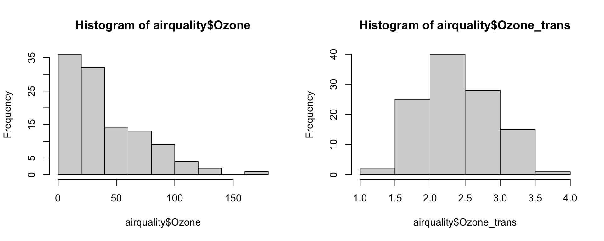
Datenexploration | Verteilung und NAs

Die Ozonwerte sind stark rechtsschief und eine erste Modellselektion zeigte, dass Ozon transformiert werden muss (4te-Wurzel).
Alle Zeilen mit NAs (81 insgesamt) werden entfernt.

Code

airquality <- airquality |>
  mutate(Ozone_trans = Ozone^0.25)

# Entfernen der NAs für die Modellauswahl später
airquality <- airquality |> drop_na()

par(mfrow = c(1,2))
hist(airquality$Ozone)
hist(airquality$Ozone_trans)

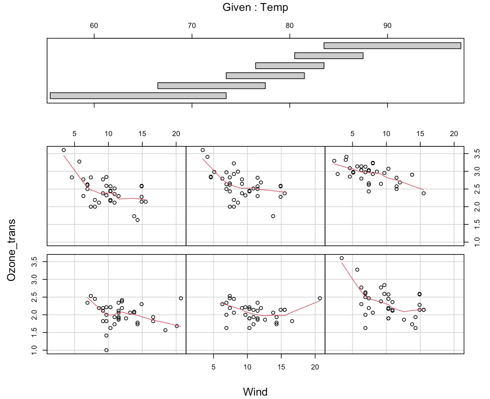
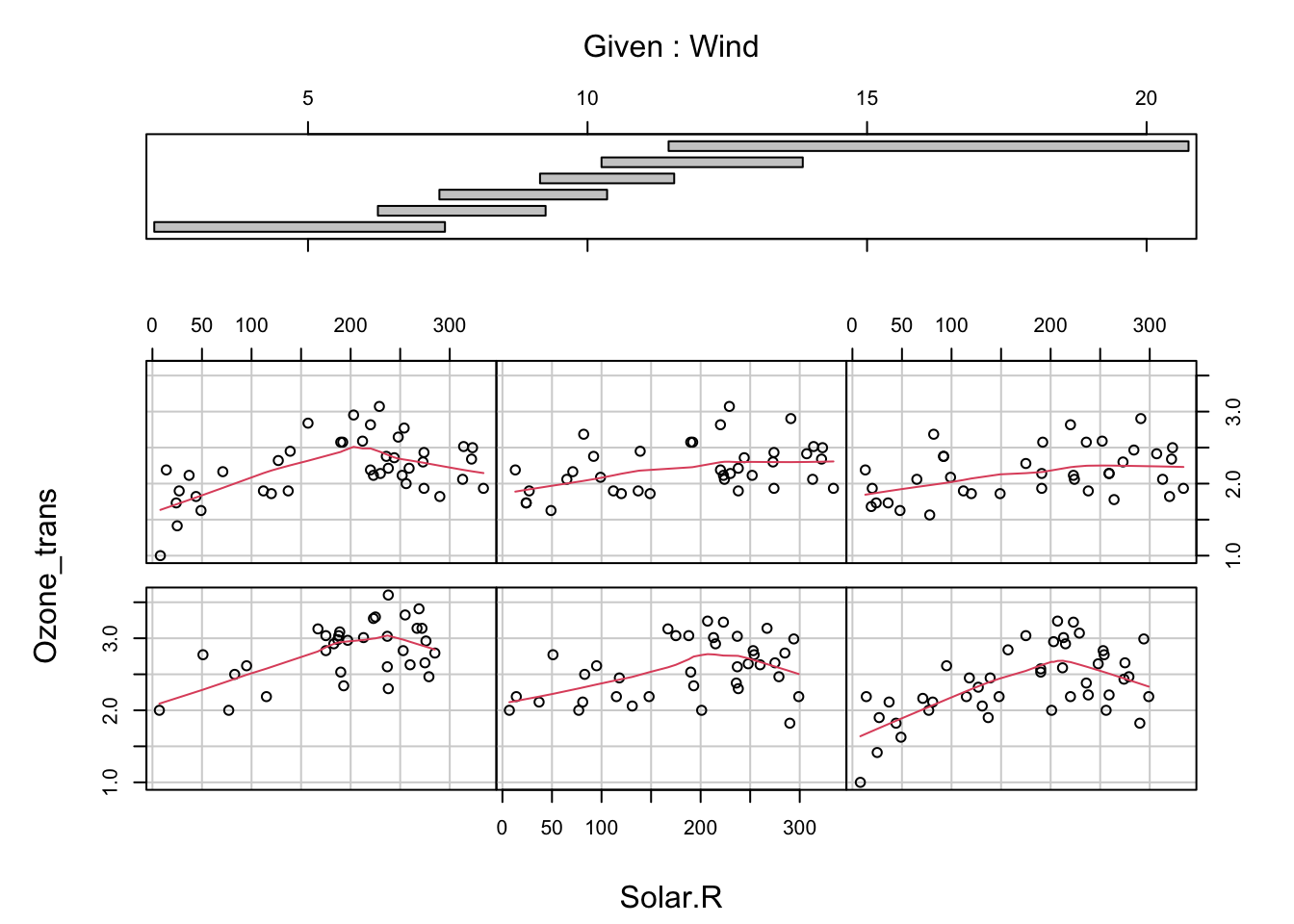
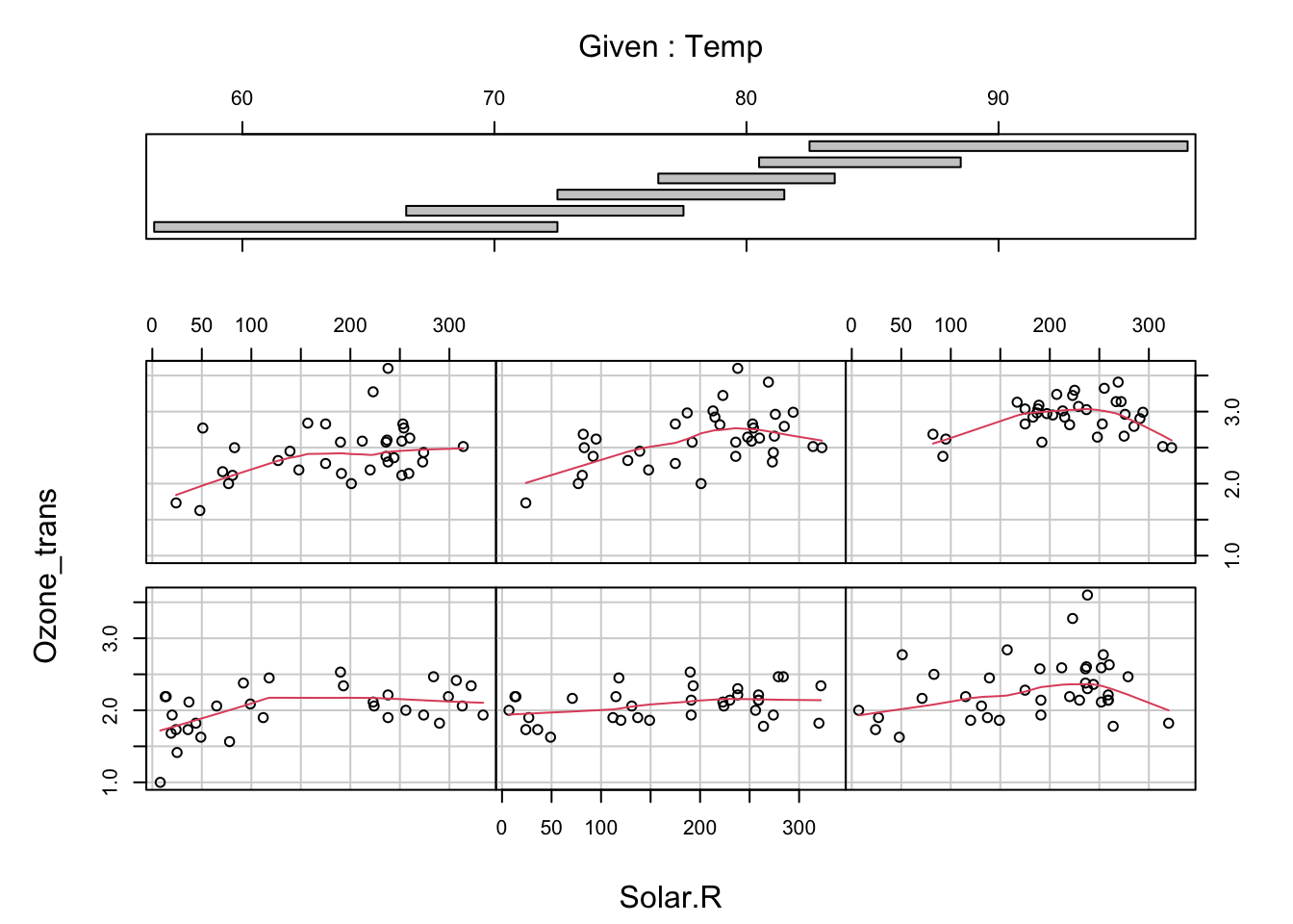
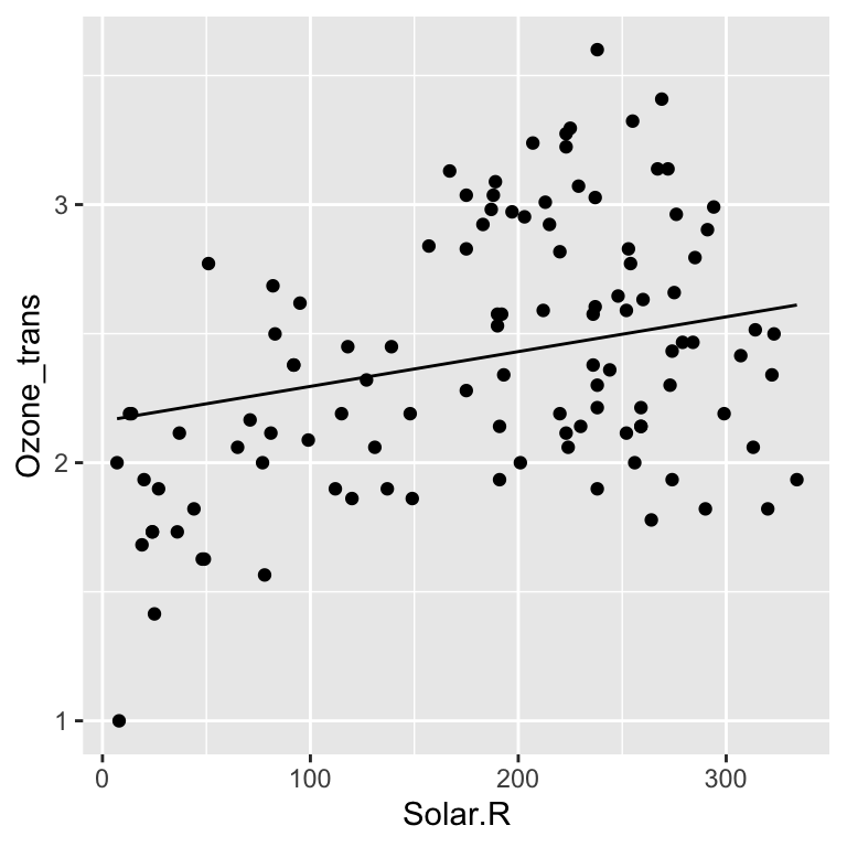
Datenexploration | Beziehungen

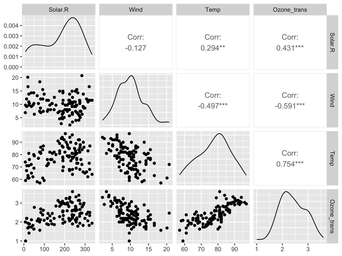
Die ggpairs() Funktion im Paket 'GGally'

GGally::ggpairs(data = airquality, columns = c(2:4, 7))  # Y zum Schluss

Datenexploration | Kolliniarität

Die vif() Funktion aus dem 'car' Paket

# Wir definieren ein Modell mit allen Variablen, aber OHNE Interaktion
mod_lm <- lm(Ozone ~ Solar.R + Wind + Temp, airquality)
car::vif(mod_lm)

 Solar.R     Wind     Temp 
1.095253 1.329070 1.431367

Keine Kovariate zeigt einen VIF-Wert > 3.
Es können daher alle im Modell bleiben.

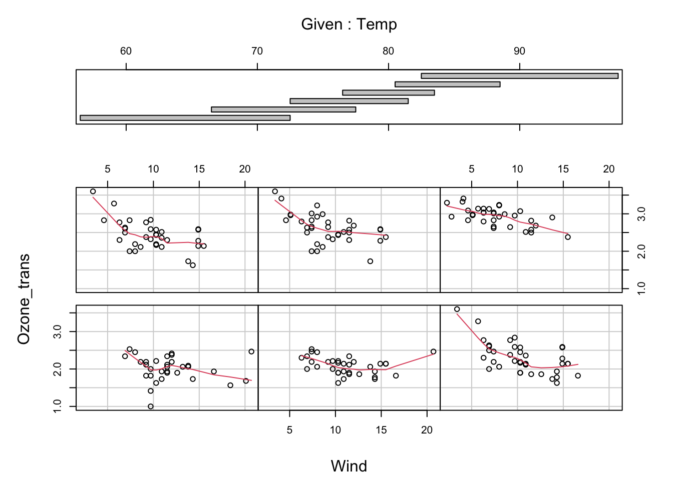
Datenexploration | Interaktionen

coplot(Ozone_trans ~ Solar.R | Wind, data = airquality, panel = panel.smooth)

coplot(Ozone_trans ~ Solar.R | Temp, data = airquality, panel = panel.smooth)

coplot(Ozone_trans ~ Wind | Temp, data = airquality, panel = panel.smooth)

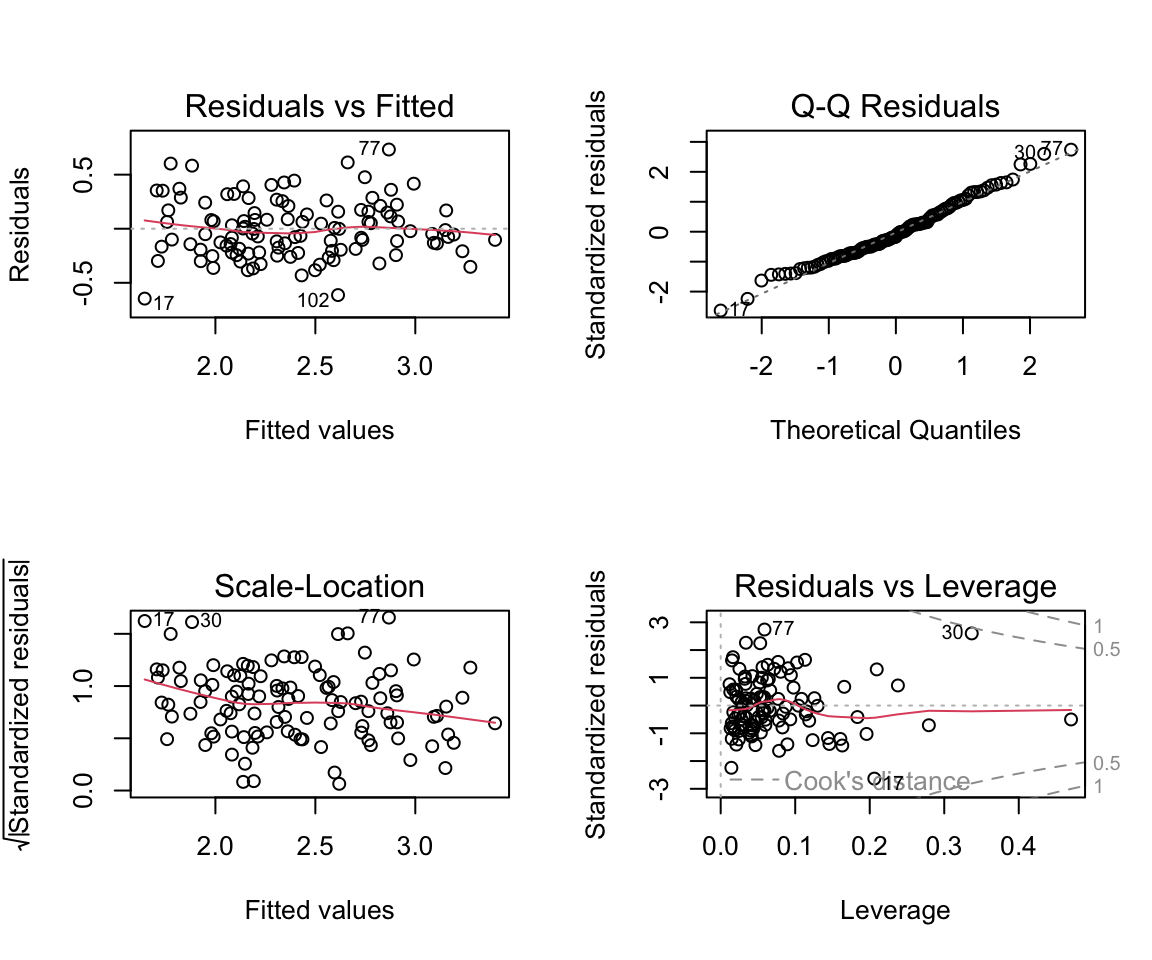
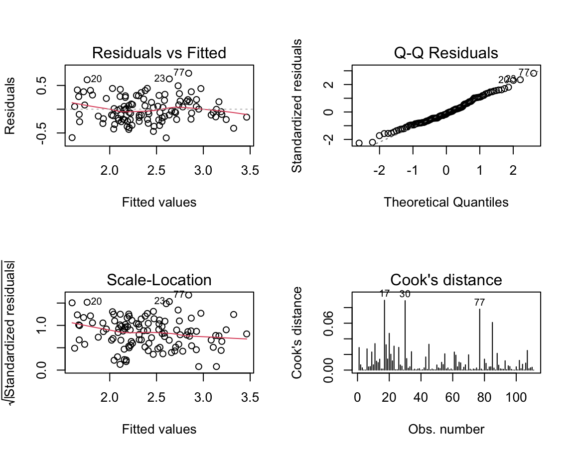
Volles Modell | Validierung

mod_full <- lm(Ozone_trans ~ Solar.R * Wind * Temp, airquality)
par(mfrow = c(2,2))
plot(mod_full)

Volles Modell | Numerischer Output

summary(mod_full)


Call:
lm(formula = Ozone_trans ~ Solar.R * Wind * Temp, data = airquality)

Residuals:
     Min       1Q   Median       3Q      Max 
-0.64623 -0.19417 -0.04487  0.16945  0.73236 

Coefficients:
                    Estimate Std. Error t value Pr(>|t|)  
(Intercept)       -1.664e+00  1.549e+00  -1.074   0.2852  
Solar.R            6.045e-03  8.431e-03   0.717   0.4750  
Wind               1.983e-01  1.275e-01   1.555   0.1231  
Temp               5.322e-02  2.118e-02   2.513   0.0135 *
Solar.R:Wind      -7.011e-04  7.438e-04  -0.943   0.3481  
Solar.R:Temp      -5.464e-05  1.118e-04  -0.489   0.6260  
Wind:Temp         -3.078e-03  1.801e-03  -1.709   0.0905 .
Solar.R:Wind:Temp  8.789e-06  1.005e-05   0.874   0.3839  
---
Signif. codes:  0 '***' 0.001 '**' 0.01 '*' 0.05 '.' 0.1 ' ' 1

Residual standard error: 0.2755 on 103 degrees of freedom
Multiple R-squared:  0.7139,    Adjusted R-squared:  0.6945 
F-statistic: 36.72 on 7 and 103 DF,  p-value: < 2.2e-16

Modellauswahl | ‘backward selection’ 1

Auswahlkriterium: AIC → `AIC()`

Schritt 1: Enfernen der 3-Wege Interaktion mit update()

mod_full <- lm(Ozone_trans ~ Solar.R * Wind * Temp, airquality)
mod_step1 <- update(mod_full, .~. - Solar.R:Wind:Temp)
AIC(mod_full, mod_step1)    # mod_step1 am besten (niedrigsten)

          df      AIC
mod_full   9 38.49526
mod_step1  8 37.31636

Schritt 2: Enfernen der drei 2-Wege-Interaktionen

mod_step2a <- update(mod_step1, .~. - Solar.R:Wind) 
mod_step2b <- update(mod_step1, .~. - Solar.R:Temp)
mod_step2c <- update(mod_step1, .~. - Wind:Temp)
AIC(mod_step1, mod_step2a, mod_step2b, mod_step2c) # mod_step2a am besten

           df      AIC
mod_step1   8 37.31636
mod_step2a  7 35.67992
mod_step2b  7 36.56975
mod_step2c  7 39.48241

Modellauswahl | ‘backward selection’ 2

Auswahlkriterium: AIC → `AIC()`

Schritt 3: Enfernen der restlichen 2-Wege-Interaktionen

mod_step3a <- update(mod_step2a, .~. - Solar.R:Temp) 
mod_step3b <- update(mod_step2a, .~. - Wind:Temp)
AIC(mod_step2a, mod_step3a, mod_step3b)   # mod_step3a am besten

           df      AIC
mod_step2a  7 35.67992
mod_step3a  6 35.38642
mod_step3b  6 39.73598

Schritt 4: Enfernen der letzten 2-Wege-Interaktion und Solar.R

# (Solar.R fehlt im Interaktionsterm, kann daher entfernt werden)
mod_step4a <- update(mod_step3a, .~. - Solar.R) 
mod_step4b <- update(mod_step3a, .~. - Wind:Temp)
AIC(mod_step3a, mod_step4a, mod_step4b)   # mod_step3a am besten

           df      AIC
mod_step3a  6 35.38642
mod_step4a  5 52.50390
mod_step4b  5 42.30848

→ Bestes Modell: mit allen 3 Kovariaten und der Wind:Temp Interaktion

Modellauswahl | Automatische Auswahl

Automatische ‘backward selection’ mit `step()`

step(mod_full)

Start:  AIC=-278.51
Ozone_trans ~ Solar.R * Wind * Temp

                    Df Sum of Sq   RSS     AIC
- Solar.R:Wind:Temp  1  0.058039 7.875 -279.69
<none>                           7.817 -278.51

Step:  AIC=-279.69
Ozone_trans ~ Solar.R + Wind + Temp + Solar.R:Wind + Solar.R:Temp + 
    Wind:Temp

               Df Sum of Sq    RSS     AIC
- Solar.R:Wind  1  0.025836 7.9008 -281.32
- Solar.R:Temp  1  0.089427 7.9644 -280.44
<none>                      7.8750 -279.69
- Wind:Temp     1  0.301181 8.1762 -277.52

Step:  AIC=-281.32
Ozone_trans ~ Solar.R + Wind + Temp + Solar.R:Temp + Wind:Temp

               Df Sum of Sq    RSS     AIC
- Solar.R:Temp  1   0.12240 8.0232 -281.62
<none>                      7.9008 -281.32
- Wind:Temp     1   0.44304 8.3439 -277.27

Step:  AIC=-281.62
Ozone_trans ~ Solar.R + Wind + Temp + Wind:Temp

            Df Sum of Sq    RSS     AIC
<none>                   8.0232 -281.62
- Wind:Temp  1   0.67153 8.6948 -274.70
- Solar.R    1   1.50797 9.5312 -264.50


Call:
lm(formula = Ozone_trans ~ Solar.R + Wind + Temp + Wind:Temp, 
    data = airquality)

Coefficients:
(Intercept)      Solar.R         Wind         Temp    Wind:Temp  
  -1.364170     0.001347     0.129726     0.050008    -0.002197

‘Optimales’ Modell | Validierung 1

Standardplots

mod_final <- lm(Ozone_trans ~ Solar.R + Wind + Temp + Wind:Temp, airquality)
par(mfrow = c(2,2))
plot(mod_final, which = 1:4)

‘Optimales’ Modell | Validierung 2

Zusätzliche Plots manuell erstellt:

Code

res <- residuals(mod_final)
fit <- fitted(mod_final)

par(mfrow = c(2,3))
hist(res)
plot(airquality$Ozone_trans ~ fit, main = "Vorhersage-Performance"); abline(0,1)
# Unabhaengigkeitscheck: Residuen vs. jede erklaerende Var.
plot(0, 0, type = "n", axes = FALSE, xlab="", ylab="")
plot(res ~ airquality$Solar.R); abline(0,0)
plot(res ~ airquality$Wind); abline(0,0)
plot(res ~ airquality$Temp); abline(0,0)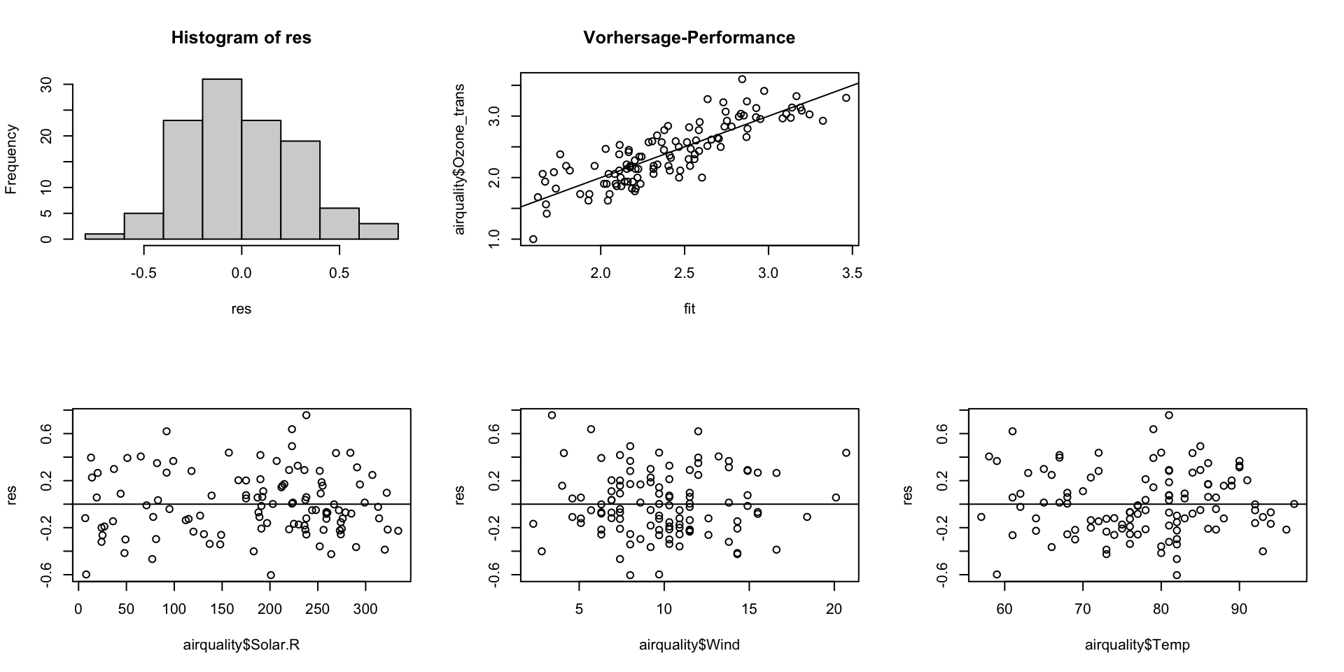

‘Optimales’ Modell | Numerischer Output

summary(mod_final)


Call:
lm(formula = Ozone_trans ~ Solar.R + Wind + Temp + Wind:Temp, 
    data = airquality)

Residuals:
    Min      1Q  Median      3Q     Max 
-0.6036 -0.2040 -0.0415  0.1940  0.7572 

Coefficients:
              Estimate Std. Error t value Pr(>|t|)    
(Intercept) -1.3641697  0.6571265  -2.076  0.04032 *  
Solar.R      0.0013472  0.0003018   4.463 2.02e-05 ***
Wind         0.1297264  0.0579676   2.238  0.02732 *  
Temp         0.0500078  0.0080260   6.231 9.56e-09 ***
Wind:Temp   -0.0021973  0.0007377  -2.979  0.00359 ** 
---
Signif. codes:  0 '***' 0.001 '**' 0.01 '*' 0.05 '.' 0.1 ' ' 1

Residual standard error: 0.2751 on 106 degrees of freedom
Multiple R-squared:  0.7064,    Adjusted R-squared:  0.6953 
F-statistic: 63.75 on 4 and 106 DF,  p-value: < 2.2e-16

Modellvisualisierung (mit plotly)

Solar.R Effekt

Code

library(modelr)
data_grid(airquality,
  Solar.R = seq_range(Solar.R, 10),
  .model = mod_final) |>
  add_predictions(model = mod_final) |>
  ggplot(aes(x = Solar.R, y = pred)) +
  geom_line() +
  geom_point(data = airquality,
    aes(y = Ozone_trans)) +
  ylab("Ozone_trans")

Kombinierter Effekt von Wind und Temp

Code

library(plotly)

df <- data_grid(airquality,
  Wind = seq_range(Wind, 50),
  Temp = seq_range(Temp, 50),
  .model = mod_final) |>
  add_predictions(model = mod_final)

df_wide <- df |>
  pivot_wider(names_from = Wind,
    values_from = pred) |>
  select(-c(1:2)) |>
  as.matrix()

p1 <- plot_ly(airquality,
  x = ~ Wind,
  y = ~ Temp,
  z = ~ Ozone_trans,
  type = "scatter3d")

add_trace(p = p1,
  z = df_wide,
  x =  seq_range(airquality$Wind, 50),
  y = seq_range(airquality$Temp, 50),
  type = "surface")

Your turn …

05:00

Multiple Regression mit `penguins`

Wir greifen nun wieder den Datensatz aus dem ‘palmerpenguins’ Paket auf, den Sie bereits aus der ANCOVA-Übung kennen.

Dieses Mal beschränken wir uns auf die Art Adelie.
Wir prüfen mittels multipler Regression, ob Schnabellänge (bill_length_mm), Schnabeltiefe (bill_depth_mm) und Flossenlänge (flipper_length_mm) das Körpergewicht (body_mass_g) erklären können – und welche dieser Variablen den größten Einfluss hat.

data(penguins, package = "palmerpenguins")
subs <- penguins |> filter(species == 'Adelie') |> 
  drop_na()
str(subs)

tibble [146 × 8] (S3: tbl_df/tbl/data.frame)
 $ species          : Factor w/ 3 levels "Adelie","Chinstrap",..: 1 1 1 1 1 1 1 1 1 1 ...
 $ island           : Factor w/ 3 levels "Biscoe","Dream",..: 3 3 3 3 3 3 3 3 3 3 ...
 $ bill_length_mm   : num [1:146] 39.1 39.5 40.3 36.7 39.3 38.9 39.2 41.1 38.6 34.6 ...
 $ bill_depth_mm    : num [1:146] 18.7 17.4 18 19.3 20.6 17.8 19.6 17.6 21.2 21.1 ...
 $ flipper_length_mm: int [1:146] 181 186 195 193 190 181 195 182 191 198 ...
 $ body_mass_g      : int [1:146] 3750 3800 3250 3450 3650 3625 4675 3200 3800 4400 ...
 $ sex              : Factor w/ 2 levels "female","male": 2 1 1 1 2 1 2 1 2 2 ...
 $ year             : int [1:146] 2007 2007 2007 2007 2007 2007 2007 2007 2007 2007 ...

Quiz 2 | Interpretation Datenepxloration

Prüfung auf Kollinearität

# pairs(subs[, c(3:5, 6)])
GGally::ggpairs(data = subs, columns = c(3:5, 6))

mod_vif <- lm(
  formula = body_mass_g ~ bill_length_mm + 
    bill_depth_mm + flipper_length_mm,
  data = subs)
car::vif(mod_vif)

   bill_length_mm     bill_depth_mm flipper_length_mm 
         1.248062          1.229067          1.175950

Was lässt sich aus dem ggpairs-Plot und den VIF-Werten schließen (Quiz ist auf der nächsten Seite)?

Quiz 2 | Interpretation Datenepxloration

Prüfung auf Kollinearität

Quiz 3 | Modellspezifikation und -auswahl

Quiz 4 | Diagnosikplots des vollen Modells

Code

mod_full <- lm(
  formula = body_mass_g ~ bill_length_mm * 
  bill_depth_mm * flipper_length_mm, 
  data = subs
)
par(mfrow = c(2,2))
plot(mod_full, which = 1:4)

Quiz 5 | Interpretation Modellauswahl

Wie ist die automatische Backward-Selection mit der step() zu interpretieren (das Quiz befindet sich am Ende)?

Automatische Backward Selection
Vergleich manuelle Backward Selection

# Automatische Modellauswahl
step(mod_full)

Start:  AIC=1700.02
body_mass_g ~ bill_length_mm * bill_depth_mm * flipper_length_mm

                                                 Df Sum of Sq      RSS    AIC
- bill_length_mm:bill_depth_mm:flipper_length_mm  1     37991 14954786 1698.4
<none>                                                        14916795 1700.0

Step:  AIC=1698.39
body_mass_g ~ bill_length_mm + bill_depth_mm + flipper_length_mm + 
    bill_length_mm:bill_depth_mm + bill_length_mm:flipper_length_mm + 
    bill_depth_mm:flipper_length_mm

                                   Df Sum of Sq      RSS    AIC
- bill_depth_mm:flipper_length_mm   1       812 14955598 1696.4
- bill_length_mm:flipper_length_mm  1      9282 14964068 1696.5
- bill_length_mm:bill_depth_mm      1     89536 15044322 1697.3
<none>                                          14954786 1698.4

Step:  AIC=1696.4
body_mass_g ~ bill_length_mm + bill_depth_mm + flipper_length_mm + 
    bill_length_mm:bill_depth_mm + bill_length_mm:flipper_length_mm

                                   Df Sum of Sq      RSS    AIC
- bill_length_mm:flipper_length_mm  1      8621 14964219 1694.5
- bill_length_mm:bill_depth_mm      1     97474 15053072 1695.3
<none>                                          14955598 1696.4

Step:  AIC=1694.48
body_mass_g ~ bill_length_mm + bill_depth_mm + flipper_length_mm + 
    bill_length_mm:bill_depth_mm

                               Df Sum of Sq      RSS    AIC
- bill_length_mm:bill_depth_mm  1     88933 15053152 1693.3
<none>                                      14964219 1694.5
- flipper_length_mm             1   1493253 16457472 1706.4

Step:  AIC=1693.35
body_mass_g ~ bill_length_mm + bill_depth_mm + flipper_length_mm

                    Df Sum of Sq      RSS    AIC
<none>                           15053152 1693.3
- flipper_length_mm  1   1500553 16553705 1705.2
- bill_length_mm     1   2447561 17500713 1713.3
- bill_depth_mm      1   3645109 18698261 1723.0


Call:
lm(formula = body_mass_g ~ bill_length_mm + bill_depth_mm + flipper_length_mm, 
    data = subs)

Coefficients:
      (Intercept)     bill_length_mm      bill_depth_mm  flipper_length_mm  
         -4270.66              54.51             144.16              16.91

# Schritt 1: Enfernen der 3-Wege Interaktion mit update()
mod_full <- lm(body_mass_g ~ bill_length_mm * bill_depth_mm * flipper_length_mm, subs)
mod_step1 <- update(mod_full, .~. - bill_length_mm:bill_depth_mm:flipper_length_mm)
AIC(mod_full, mod_step1) # mod_step1 am besten (niedrigster AIC)

          df      AIC
mod_full   9 2116.351
mod_step1  8 2114.723

# Schritt 2: Enfernen der drei 2-Wege-Interaktionen
mod_step2a <- update(mod_step1, .~. - bill_length_mm:bill_depth_mm)
mod_step2b <- update(mod_step1, .~. - bill_length_mm:flipper_length_mm)
mod_step2c <- update(mod_step1, .~. - bill_depth_mm:flipper_length_mm)
AIC(mod_step1, mod_step2a, mod_step2b, mod_step2c) # alle sehr ähnlich, mod_step2c am niedrigsten

           df      AIC
mod_step1   8 2114.723
mod_step2a  7 2113.594
mod_step2b  7 2112.813
mod_step2c  7 2112.731

# Schritt 3: Enfernen der restlichen 2-Wege-Interaktionen
mod_step3a <- update(mod_step2c, .~. - bill_length_mm:bill_depth_mm)
mod_step3b <- update(mod_step2c, .~. - bill_length_mm:flipper_length_mm)
AIC(mod_step2c, mod_step3a, mod_step3b)   # mod_step3b am niedrigsten

           df      AIC
mod_step2c  7 2112.731
mod_step3a  6 2111.679
mod_step3b  6 2110.815

# Schritt 4: Enfernen der letzten 2-Wege-Interaktion und flipper_length_mm
# (flipper_length_mm fehlt im Interaktionsterm, kann daher entfernt werden)
mod_step4a <- update(mod_step3b, .~. - bill_length_mm:bill_depth_mm)
mod_step4b <- update(mod_step3b, .~. - flipper_length_mm)
AIC(mod_step3b, mod_step4a, mod_step4b) # mod_step4a am niedrigsten

           df      AIC
mod_step3b  6 2110.815
mod_step4a  5 2109.680
mod_step4b  5 2122.702

# Schritt 5: Enfernen der Einzelterme jetzt möglich
mod_step5a <- update(mod_step4a, .~. - bill_length_mm)
mod_step5b <- update(mod_step4a, .~. - bill_depth_mm)
mod_step5c <- update(mod_step4a, .~. - flipper_length_mm)
AIC(mod_step4a, mod_step5a, mod_step5b, mod_step5c) # mod_step4a deutlich am niedrigsten (Diff. > 2)

           df      AIC
mod_step4a  5 2109.680
mod_step5a  4 2129.675
mod_step5b  4 2139.339
mod_step5c  4 2121.553

# Bestes Modell
summary(mod_step4a)


Call:
lm(formula = body_mass_g ~ bill_length_mm + bill_depth_mm + flipper_length_mm, 
    data = subs)

Residuals:
    Min      1Q  Median      3Q     Max 
-816.24 -201.66  -11.49  196.83  885.34 

Coefficients:
                   Estimate Std. Error t value Pr(>|t|)    
(Intercept)       -4270.655    811.928  -5.260 5.20e-07 ***
bill_length_mm       54.512     11.345   4.805 3.89e-06 ***
bill_depth_mm       144.157     24.584   5.864 3.03e-08 ***
flipper_length_mm    16.915      4.496   3.762 0.000246 ***
---
Signif. codes:  0 '***' 0.001 '**' 0.01 '*' 0.05 '.' 0.1 ' ' 1

Residual standard error: 325.6 on 142 degrees of freedom
Multiple R-squared:  0.5064,    Adjusted R-squared:  0.496 
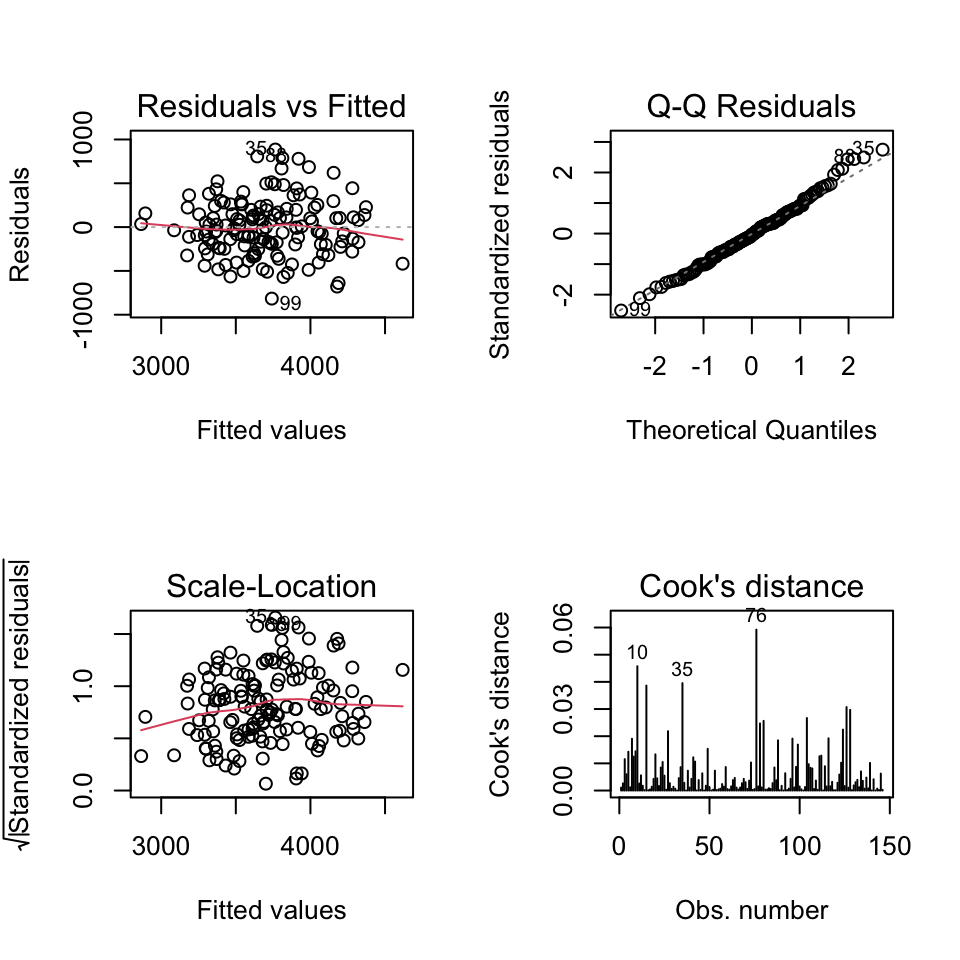
F-statistic: 48.57 on 3 and 142 DF,  p-value: < 2.2e-16

Quiz 6 | Diagnosikplots des finalen Modells

Code

mod_final <- lm(
  formula = body_mass_g ~ bill_length_mm + 
  bill_depth_mm + flipper_length_mm, 
  data = subs
)
par(mfrow = c(2,2))
plot(mod_final, which = 1:4)

Quiz 7 | Interpretation numerischer Output

summary(mod_final)


Call:
lm(formula = body_mass_g ~ bill_length_mm + bill_depth_mm + flipper_length_mm, 
    data = subs)

Residuals:
    Min      1Q  Median      3Q     Max 
-816.24 -201.66  -11.49  196.83  885.34 

Coefficients:
                   Estimate Std. Error t value Pr(>|t|)    
(Intercept)       -4270.655    811.928  -5.260 5.20e-07 ***
bill_length_mm       54.512     11.345   4.805 3.89e-06 ***
bill_depth_mm       144.157     24.584   5.864 3.03e-08 ***
flipper_length_mm    16.915      4.496   3.762 0.000246 ***
---
Signif. codes:  0 '***' 0.001 '**' 0.01 '*' 0.05 '.' 0.1 ' ' 1

Residual standard error: 325.6 on 142 degrees of freedom
Multiple R-squared:  0.5064,    Adjusted R-squared:  0.496 
F-statistic: 48.57 on 3 and 142 DF,  p-value: < 2.2e-16

Fragen..??

Total konfus?

Buchkapitel zum Nachlesen

The R Book von M.J. Crawley:
- Kapitel 10.13 Multiple Regression
Experimental Design and Data Analysis for Biologists von G.P. Quinn & M.J. Keough:
- Kapitel 6.1 Multiple linear regression analysis

Total gelangweilt?

Dann testen Sie doch Ihr Wissen in folgendem Abschlussquiz…

Abschlussquiz

Bei weiteren Fragen: saskia.otto(at)uni-hamburg.de

Diese Arbeit is lizenziert unter einer Creative Commons Attribution-ShareAlike 4.0 International License mit Ausnahme der entliehenen und mit Quellenangabe versehenen Abbildungen.

Multiple lineare Regression und Modellselektion

Lernziele

Am Ende dieser VL- und Übungseinheit werden Sie

Regression mit ≥ 2 Kovariaten

Multiple Regression | Ziel

Multiple Regression | Gleichung

Multiple Regression | Neu

Zusätzliche Annahmen

Problem der Kollinearität

Problem der Kollinearität | Demo

Prüfen auf Kollinearität

VIF-Wert

Weitere Datenexploration

Parameterschätzung

Signifikanztests | Partielle Koeffizienten

Anpassung des Bestimmtheitsmaß

Lösung: korrigiertes Bestimmtheitsmaß

Modellauswahl

Ausgangssituation

Sparsamkeitsprinzip

Oder Ockhams Rasiermesser

Kriterien der Modellauswahl

‘All subsets selection’

‘Stepwise selection’

‘Backward selection’ | 1

Wir starten mit allen Variablen und Interaktionen

‘Backward selection’ | 2

Schrittweises Entfernen

‘Backward selection’ | 3

Schrittweises Entfernen

‘Backward selection’ | 4

Schrittweises Entfernen

Your turn …

Quiz 1 | Formelschreibweise

Praxisbeispiel in R

Beispiel in R

‘airquality’-Datensatz

Datenexploration | Verteilung und NAs

Datenexploration | Beziehungen

Datenexploration | Kolliniarität

Datenexploration | Interaktionen

Volles Modell | Validierung

Volles Modell | Numerischer Output

Modellauswahl | ‘backward selection’ 1

Auswahlkriterium: AIC → AIC()

Modellauswahl | ‘backward selection’ 2

Auswahlkriterium: AIC → AIC()

Modellauswahl | Automatische Auswahl

Automatische ‘backward selection’ mit step()

‘Optimales’ Modell | Validierung 1

‘Optimales’ Modell | Validierung 2

‘Optimales’ Modell | Numerischer Output

Modellvisualisierung (mit plotly)

Your turn …

Multiple Regression mit penguins

Quiz 2 | Interpretation Datenepxloration

Prüfung auf Kollinearität

Quiz 2 | Interpretation Datenepxloration

Prüfung auf Kollinearität

Quiz 3 | Modellspezifikation und -auswahl

Quiz 4 | Diagnosikplots des vollen Modells

Quiz 5 | Interpretation Modellauswahl

Quiz 6 | Diagnosikplots des finalen Modells

Quiz 7 | Interpretation numerischer Output

Fragen..??

Total konfus?

Buchkapitel zum Nachlesen

Total gelangweilt?

Abschlussquiz

Regression mit
≥ 2 Kovariaten

Auswahlkriterium: AIC → `AIC()`

Auswahlkriterium: AIC → `AIC()`

Automatische ‘backward selection’ mit `step()`

Multiple Regression mit `penguins`