# library(ggplot2) # oder: library(tidyverse)
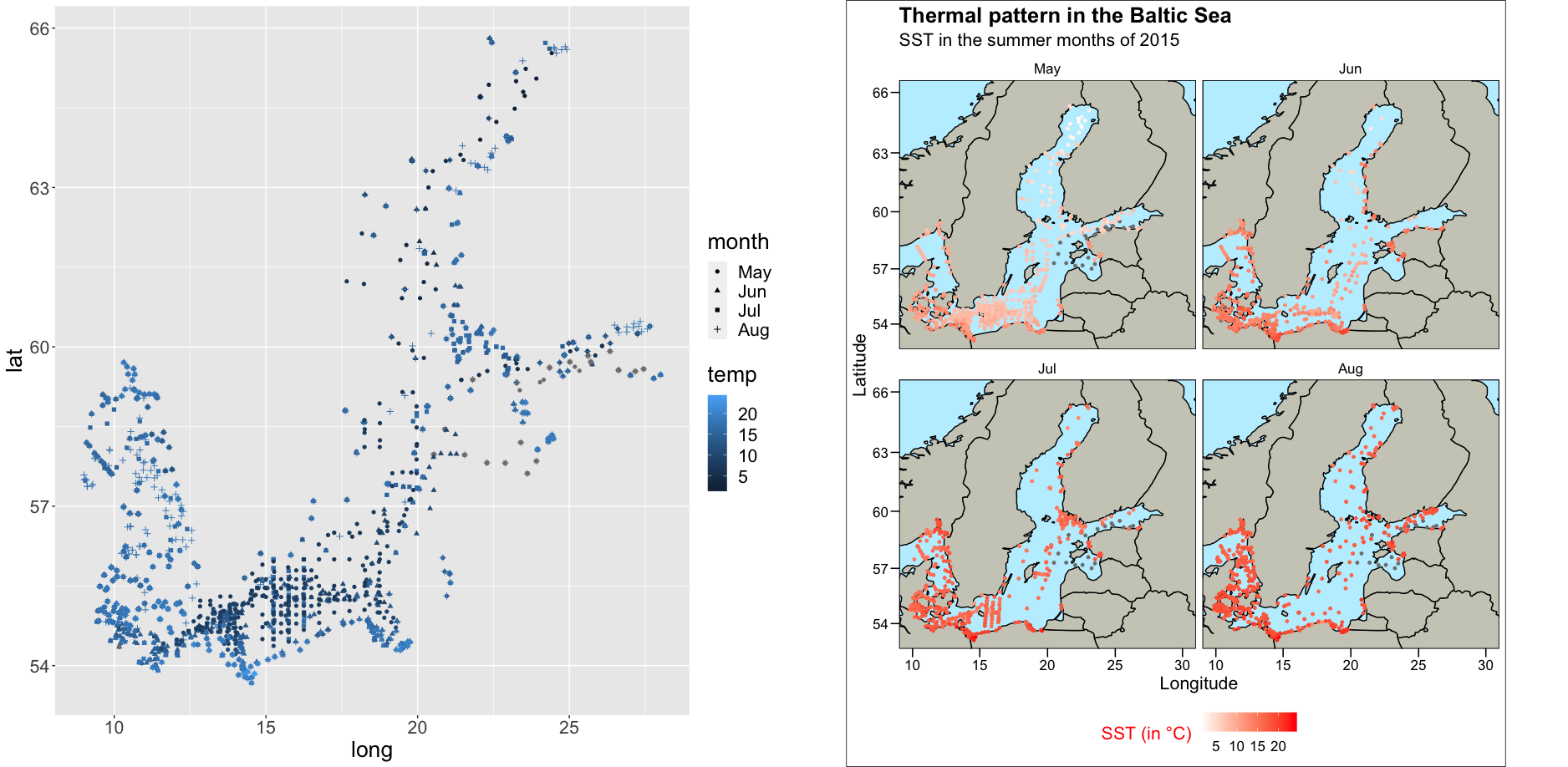
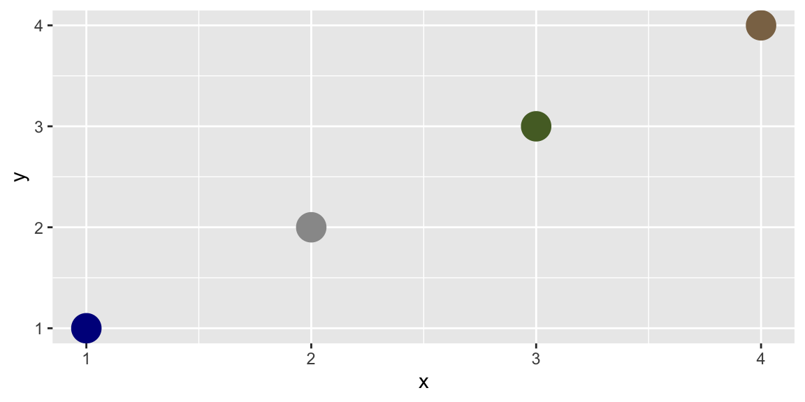
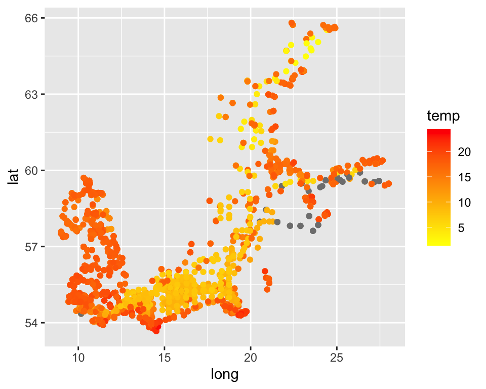
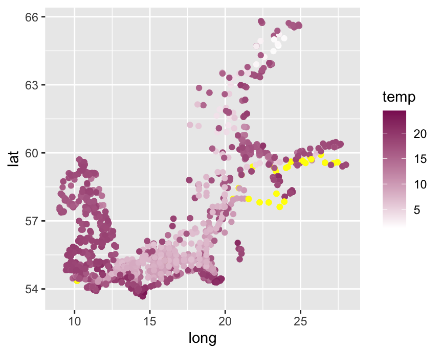
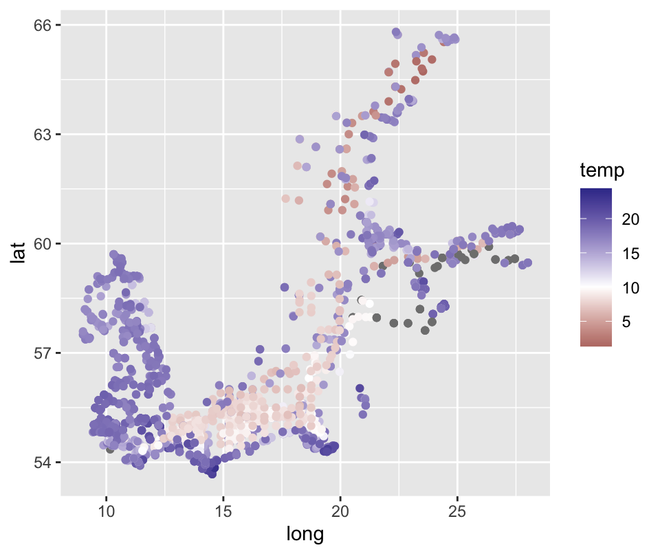
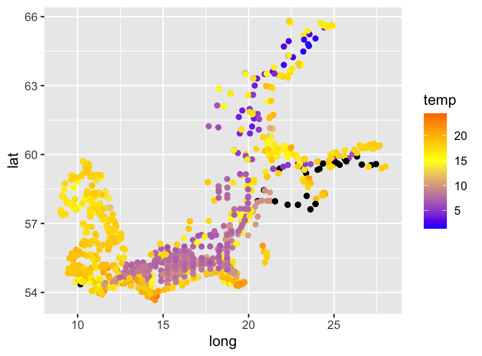
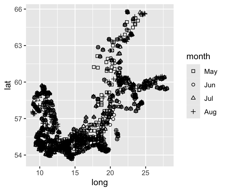
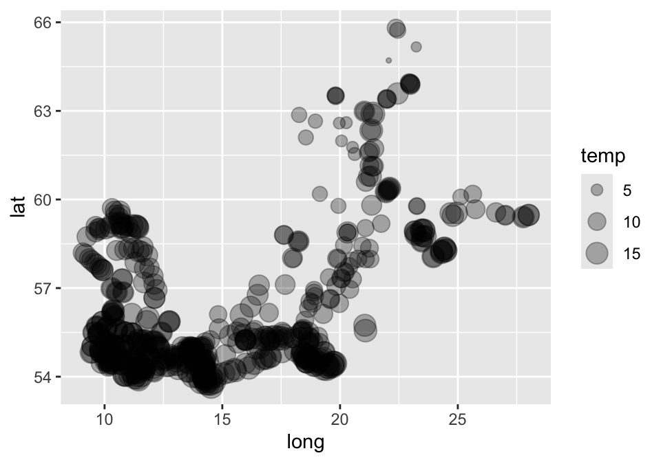
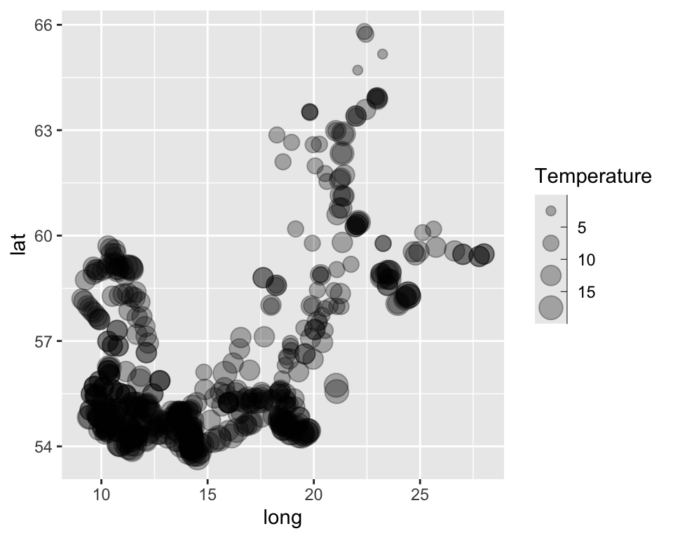
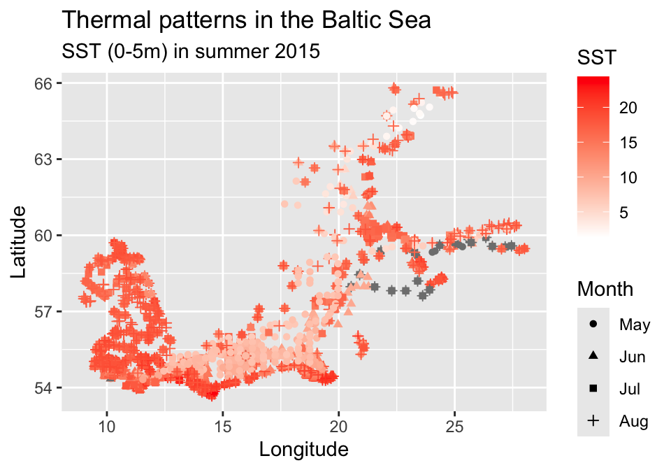
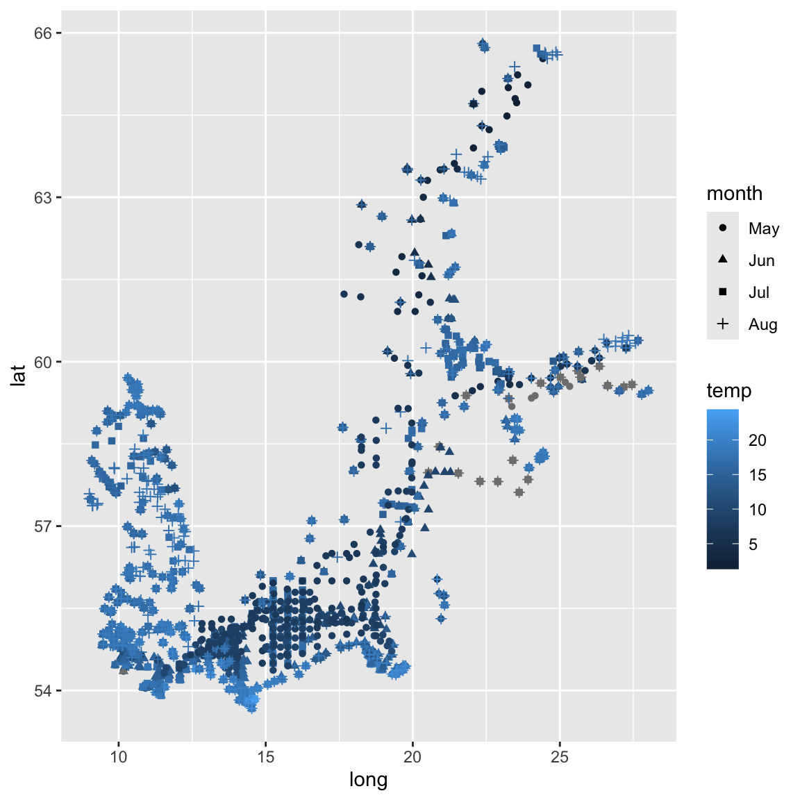
p1 <- ggplot(sst_sum, aes(long, lat)) +
geom_point(aes(colour = temp, shape = month))
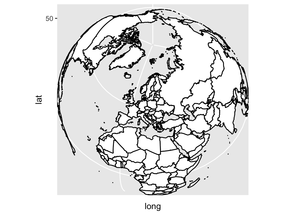
world <- map_data("world")
worldmap <- ggplot(world, aes(x = long, y = lat)) +
geom_polygon(aes(group = group), fill = "ivory3", colour = "black")
baltic <- worldmap + coord_map("ortho", xlim = c(10, 30), ylim = c(54,66))
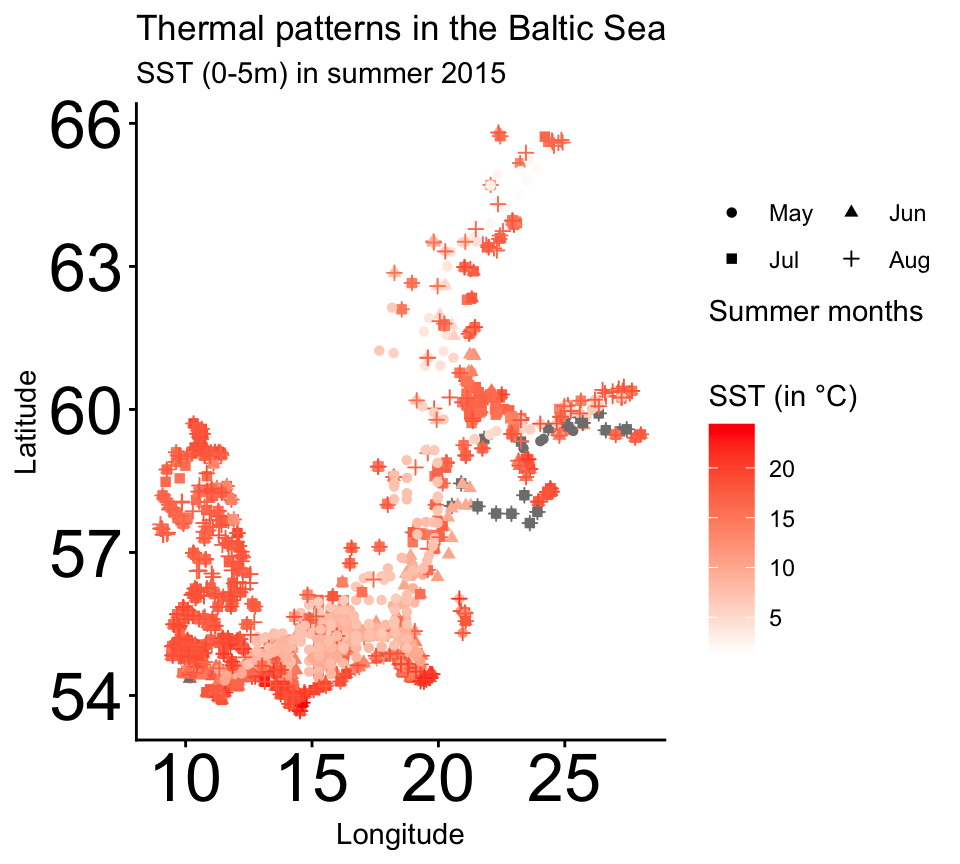
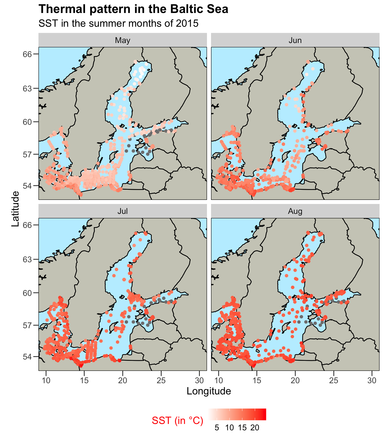
p2 <- baltic +
geom_point(data = sst_sum,
aes(x = long, y = lat, colour = temp), size = 1) +
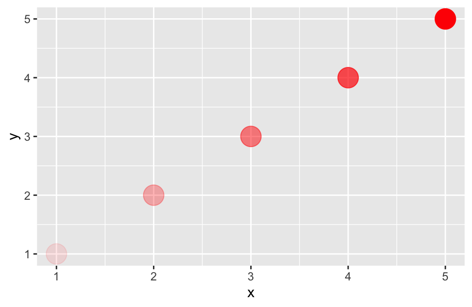
scale_colour_gradient(low = "white", high = "red") +
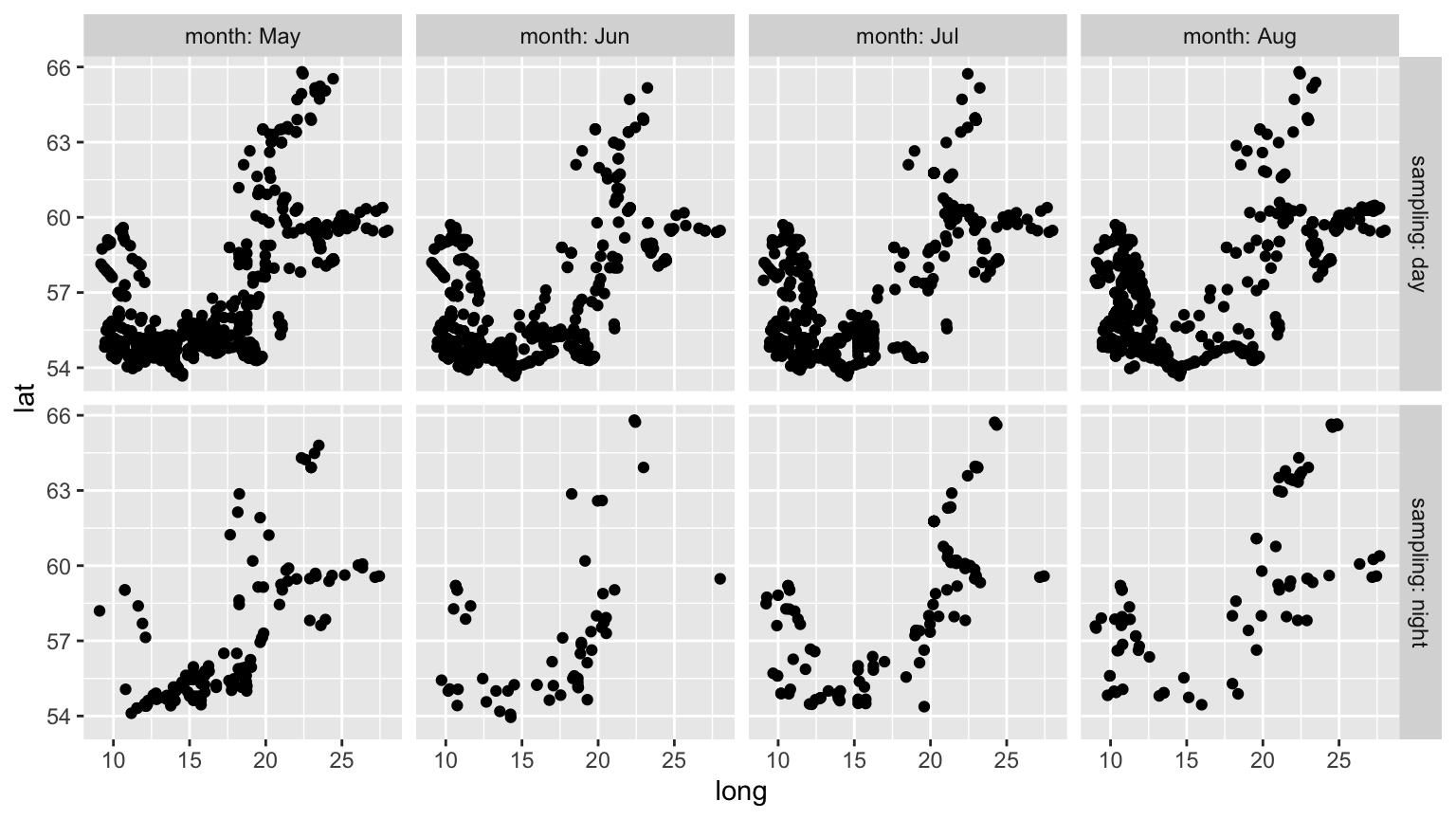
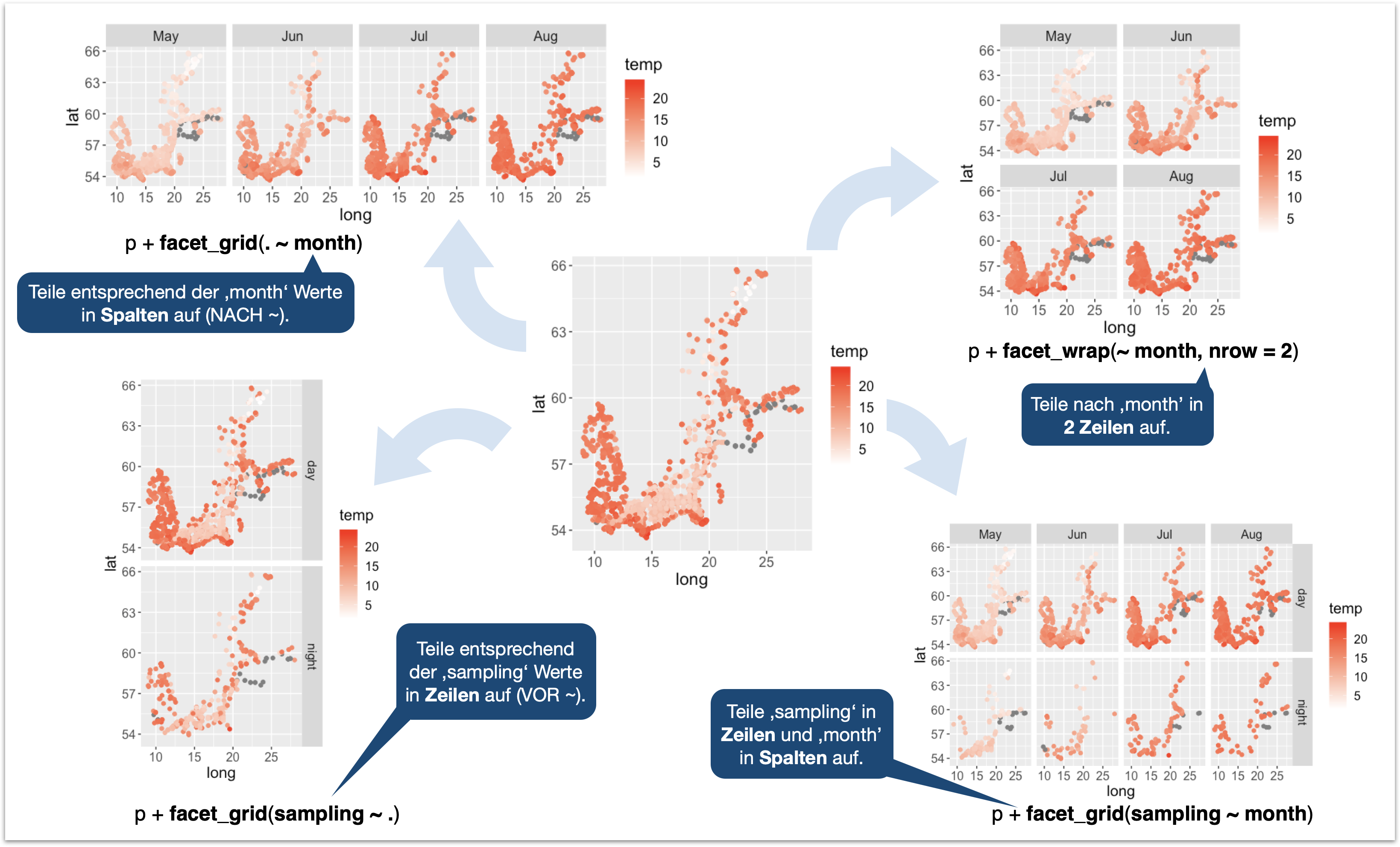
facet_wrap(~month) +
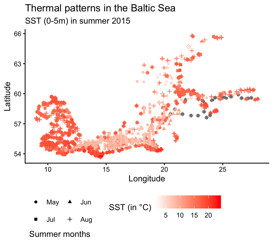
labs(x = "Longitude", y = "Latitude",
title = "Thermal pattern in the Baltic Sea",
subtitle = "SST in the summer months of 2015") +
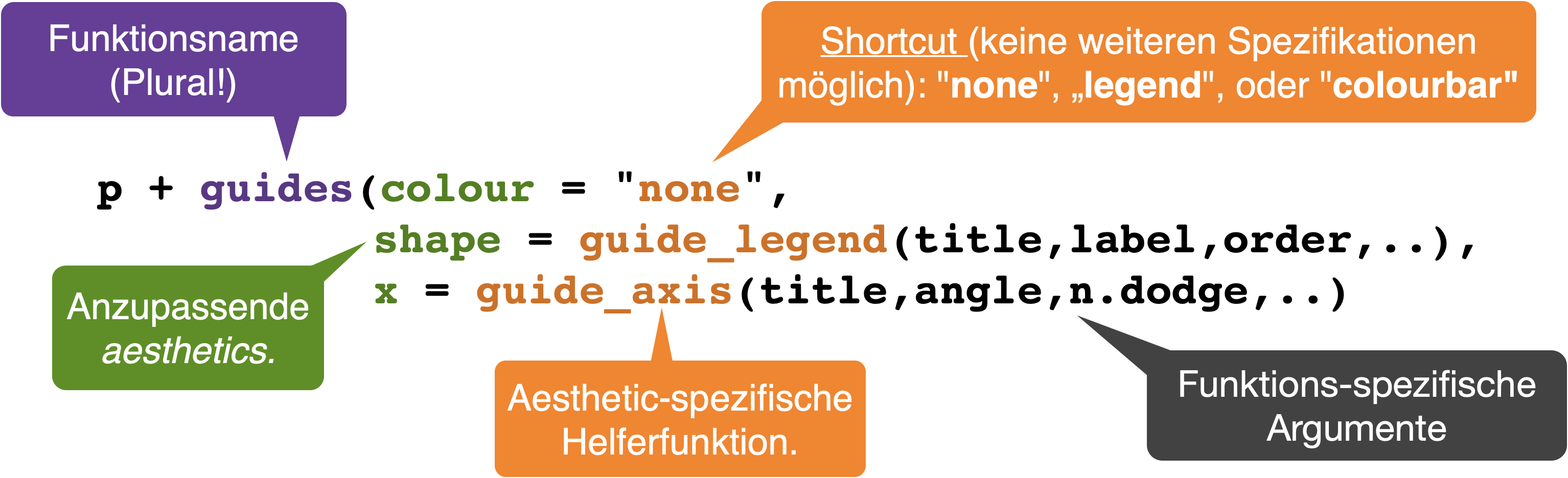
guides(colour = guide_colourbar(title = "SST (in °C)")) +
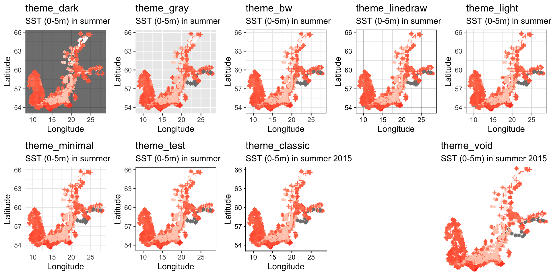
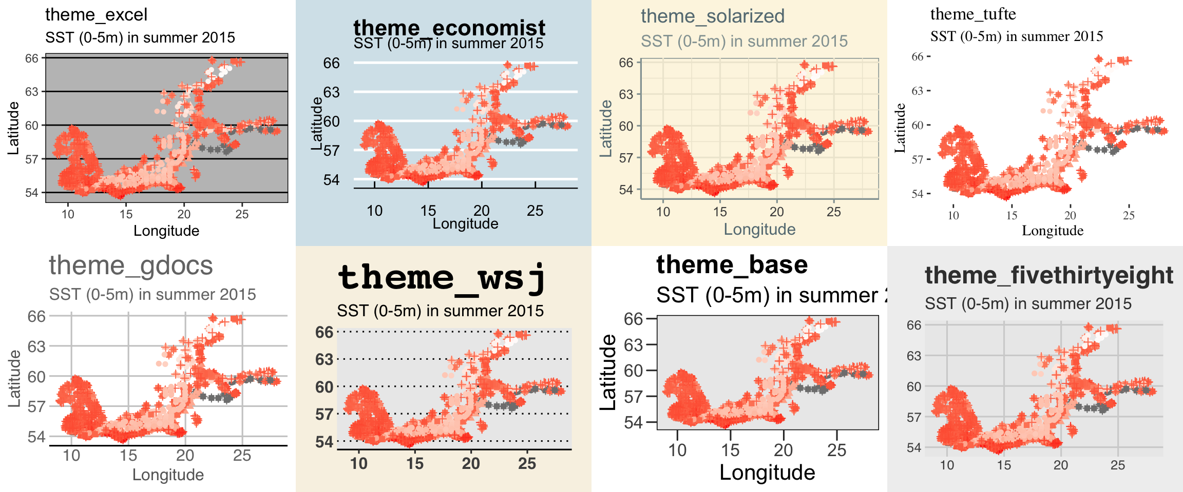
ggthemes::theme_base(base_size = 11) +
theme(
legend.position = "bottom",
legend.title.align = 1,
legend.title = element_text(colour = "red", angle = 0),
panel.background = element_rect(fill = "lightblue1")
)
gridExtra::grid.arrange(p1, p2, nrow=1)