Datenanalyse mit R

5 - Data wrangling - 2.Tidy Daten

Saskia A. Otto
BSH 11/02 - 13/02 2019

2. Tidy data

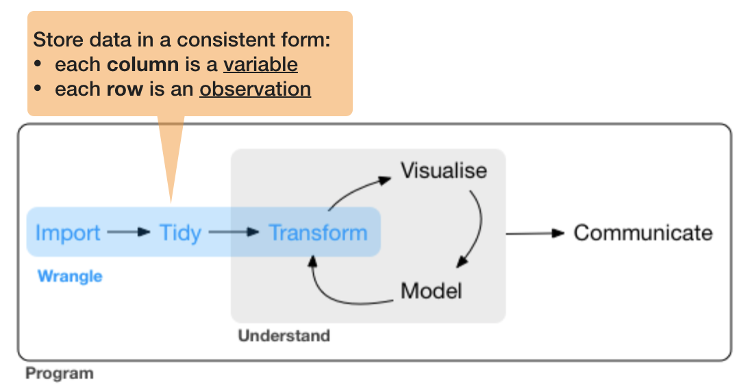
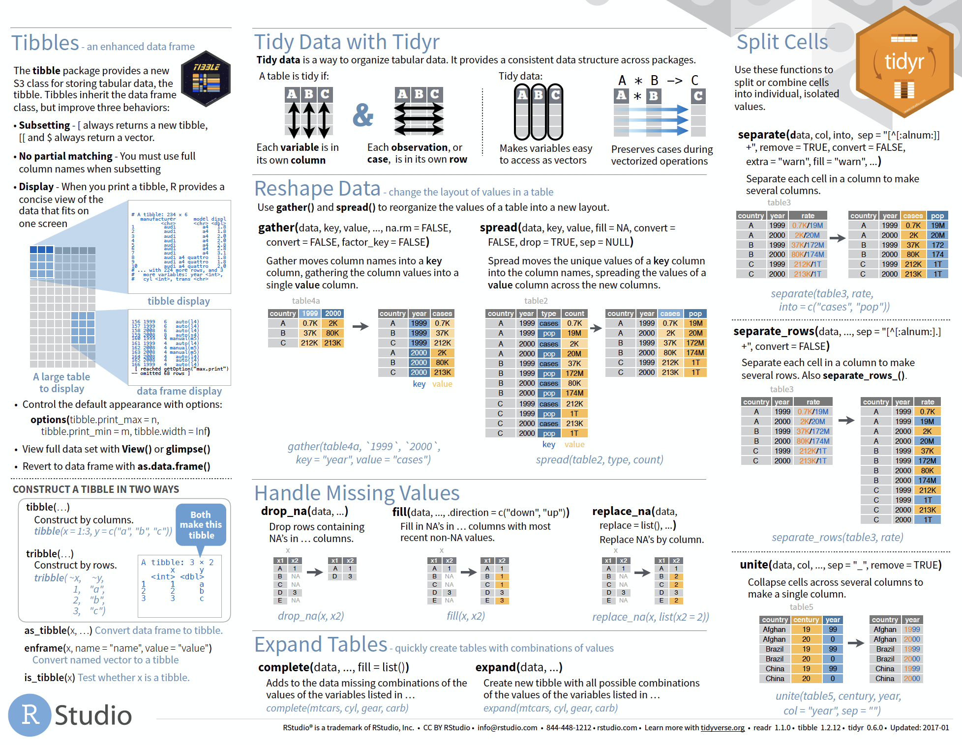
So what is 'tidy' data?

A way to organize tabular data

So what is 'tidy' data?

A way to organize tabular data

source: Data Import cheat sheet (licensed under CC-BY-SA)

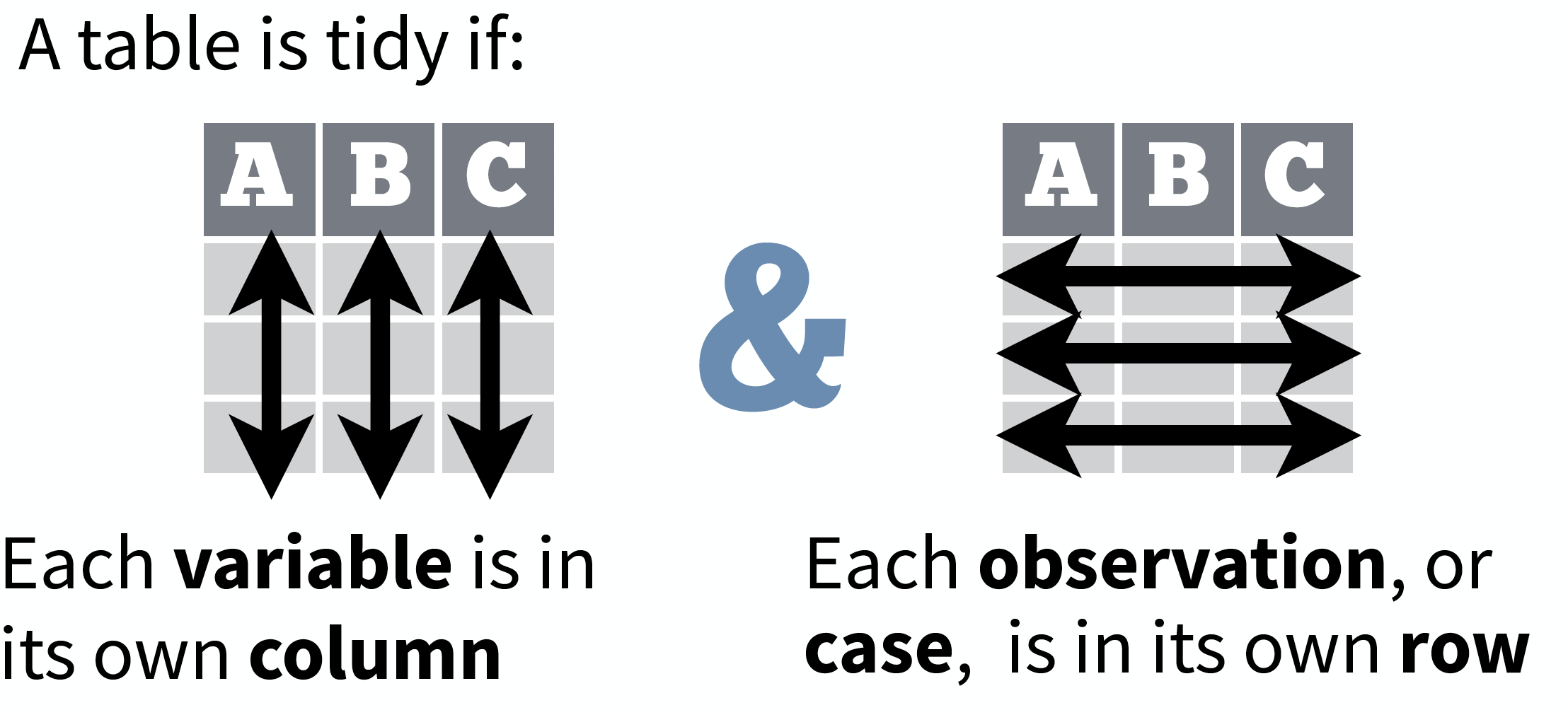
So what is 'tidy' data?

A way to organize tabular data
Provides a consistent data structure across packages.
Is easy to aggregate, visualise and model (i.e. works well with dplyr, ggplot, and lm)
Complements R’s vectorized operations --> R will automatically preserve observations as you manipulate variables.

So what is 'tidy' data?

A way to organize tabular data
Provides a consistent data structure across packages.
Is easy to aggregate, visualise and model (i.e. works well with dplyr, ggplot, and lm)
Complements R’s vectorized operations --> R will automatically preserve observations as you manipulate variables.

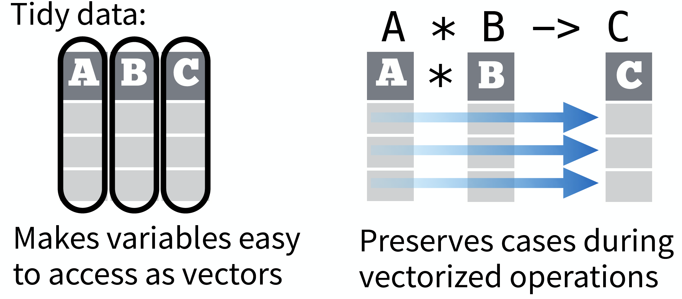
source: Data Import cheat sheet (licensed under CC-BY-SA)

So what is 'tidy' data?

A way to organize tabular data
Provides a consistent data structure across packages.
Is easy to aggregate, visualise and model (i.e. works well with dplyr, ggplot, and lm)
Complements R’s vectorized operations --> R will automatically preserve observations as you manipulate variables.
Something than many people have intuitively applied
But Hadley Wickham developed a whole framework around this concept and with the tidverse packages, and particularly 'tidyr', it is much easier to adopt

plot of chunk unnamed-chunk-1

Another example with the hydrographical data from ICES

What can be potential issues with such a table?

plot of chunk unnamed-chunk-2

An example with the hydrographical data from ICES

What can be potential issues with such a table?

plot of chunk unnamed-chunk-3

Where should the coordinates per station be added? In an extra table?
Where should the date be added? On top of the station names?
What to do with the other parameters, salinity and oxygen? Different files?
Not clear that the values represent temperature!

Solution: Restructure the table again

plot of chunk unnamed-chunk-4

Long vs. wide data

The 'long' data format is considered more tidy as
- each observation (here temperature measurement) is in its own row
- each variable has its own column → station and temperature are not mixed anymore!
BUT: some functions require the data to be in a wide format --> you need to adjust your data table in that case

2. Tidy data - How to change between data formats?

'tidyr' provides two functions for that:

gather() and
spread()

`gather()`

Moves column names into a key column, gathering the column values into a single value column. plot of chunk unnamed-chunk-5

`spread()`

Moves the unique values of a key column into the column names, spreading the values of a value column across the new columns. plot of chunk unnamed-chunk-6

In the R console you would write for the hydrographical example

cruise <- tibble(pressure = 1:5, station_1 = c(14.1,14.0,14.0,13.9,13.8),
  station_2 = c(15.3,15.4,15.2,15.0,14.9))
cruise
# Make tibble long
cruise_long <- gather(cruise, station_1, station_2, key = "station", value = "temp")
cruise_long
# Reshape tibble back into wide format
cruise_wide <- spread(cruise_long, station, temp)
cruise_wide # same as cruise!

TRY IT YOURSELF!

Your turn...

Quiz 1: Restructuring data formats

Make the following temperature data long and then wide again:

(cruise <- tibble(pressure = 1:5, station_1 = c(14.1,14.0,14.0,13.9,13.8),
  station_2 = c(15.3,15.4,15.2,15.0,14.9)) )

## # A tibble: 5 x 3
##   pressure station_1 station_2
##      <int>     <dbl>     <dbl>
## 1        1      14.1      15.3
## 2        2      14        15.4
## 3        3      14        15.2
## 4        4      13.9      15  
## 5        5      13.8      14.9

Solution: Restructuring data formats

# Make tibble long
cruise_long <- gather(cruise, station_1, station_2, 
  key = "station", value = "temp")
cruise_long

## # A tibble: 10 x 3
##    pressure station    temp
##       <int> <chr>     <dbl>
##  1        1 station_1  14.1
##  2        2 station_1  14  
##  3        3 station_1  14  
##  4        4 station_1  13.9
##  5        5 station_1  13.8
##  6        1 station_2  15.3
##  7        2 station_2  15.4
##  8        3 station_2  15.2
##  9        4 station_2  15  
## 10        5 station_2  14.9

Solution: Restructuring data formats

# Reshape tibble back into wide format
cruise_wide <- spread(cruise_long, station, temp)
cruise_wide # same as cruise!

## # A tibble: 5 x 3
##   pressure station_1 station_2
##      <int>     <dbl>     <dbl>
## 1        1      14.1      15.3
## 2        2      14        15.4
## 3        3      14        15.2
## 4        4      13.9      15  
## 5        5      13.8      14.9

2. Tidy data - Handling missing values and other replacements

Handling missing values (NAs)

Leave them in and accomodate algorithm to missing data, e.g. missing values are skipped during calculations like "pairwise deletion"; can cause problems
Delete rows/columns
Interpolate missing values
- replace NAs by mean/median (advantage median: distribution can be skewed)
- replace NAs by regression (linear interpolation)

Checking for NAs

You can apply the function is.na() to single vectors and single variables in a data frame as you learned in lecture 2. Here an example with the ICES dataset

is.na(hydro$temp)

##    [1] FALSE FALSE FALSE FALSE FALSE FALSE FALSE FALSE FALSE FALSE FALSE
##   [12] FALSE FALSE FALSE FALSE FALSE FALSE FALSE FALSE FALSE FALSE FALSE
##   [23] FALSE FALSE  TRUE FALSE FALSE FALSE FALSE FALSE FALSE FALSE  TRUE
##   [34] FALSE FALSE FALSE  TRUE  TRUE  TRUE  TRUE  TRUE  TRUE  TRUE  TRUE
##   [45]  TRUE  TRUE  TRUE  TRUE  TRUE  TRUE  TRUE  TRUE  TRUE  TRUE  TRUE
##   [56]  TRUE  TRUE FALSE FALSE FALSE FALSE FALSE FALSE FALSE FALSE FALSE
##   [67] FALSE FALSE FALSE FALSE FALSE FALSE FALSE FALSE FALSE FALSE FALSE
##   [78] FALSE FALSE FALSE FALSE FALSE FALSE FALSE  TRUE FALSE FALSE  TRUE
##   [89] FALSE FALSE  TRUE FALSE FALSE FALSE FALSE FALSE FALSE FALSE FALSE
##  [100] FALSE FALSE FALSE FALSE FALSE FALSE FALSE FALSE FALSE FALSE FALSE
##  [111] FALSE FALSE FALSE FALSE FALSE FALSE FALSE FALSE FALSE FALSE FALSE
##  [122] FALSE FALSE FALSE FALSE  TRUE  TRUE  TRUE  TRUE  TRUE  TRUE  TRUE
##  [133]  TRUE  TRUE  TRUE  TRUE FALSE FALSE  TRUE FALSE FALSE FALSE FALSE
##  [144] FALSE FALSE FALSE FALSE FALSE FALSE  TRUE FALSE FALSE FALSE FALSE
##  [155] FALSE  TRUE FALSE FALSE FALSE FALSE  TRUE FALSE FALSE FALSE FALSE
##  [166] FALSE FALSE FALSE FALSE FALSE  TRUE FALSE FALSE FALSE FALSE FALSE
##  [177] FALSE FALSE FALSE FALSE FALSE FALSE FALSE FALSE FALSE FALSE FALSE
##  [188] FALSE FALSE FALSE FALSE FALSE FALSE FALSE FALSE FALSE FALSE FALSE
##  [199] FALSE FALSE FALSE FALSE FALSE FALSE FALSE FALSE FALSE FALSE FALSE
##  [210] FALSE FALSE FALSE FALSE FALSE FALSE FALSE FALSE FALSE FALSE FALSE
##  [221] FALSE FALSE FALSE FALSE FALSE FALSE FALSE FALSE FALSE FALSE FALSE
##  [232] FALSE FALSE FALSE FALSE FALSE FALSE FALSE FALSE FALSE FALSE FALSE
##  [243] FALSE FALSE FALSE FALSE FALSE FALSE FALSE FALSE FALSE FALSE FALSE
##  [254] FALSE FALSE FALSE FALSE FALSE FALSE FALSE FALSE FALSE FALSE FALSE
##  [265] FALSE FALSE FALSE FALSE FALSE FALSE FALSE FALSE FALSE FALSE FALSE
##  [276] FALSE FALSE FALSE FALSE FALSE FALSE FALSE FALSE FALSE FALSE FALSE
##  [287] FALSE FALSE FALSE FALSE FALSE FALSE FALSE FALSE FALSE FALSE FALSE
##  [298] FALSE FALSE FALSE FALSE FALSE FALSE FALSE FALSE FALSE FALSE FALSE
##  [309] FALSE FALSE FALSE FALSE FALSE FALSE FALSE FALSE FALSE FALSE FALSE
##  [320] FALSE FALSE FALSE FALSE FALSE FALSE FALSE FALSE FALSE FALSE FALSE
##  [331] FALSE FALSE FALSE FALSE FALSE FALSE FALSE FALSE FALSE FALSE FALSE
##  [342] FALSE FALSE FALSE FALSE FALSE FALSE FALSE FALSE FALSE FALSE FALSE
##  [353] FALSE FALSE FALSE FALSE FALSE FALSE FALSE FALSE FALSE FALSE FALSE
##  [364] FALSE FALSE FALSE FALSE FALSE FALSE FALSE FALSE FALSE FALSE FALSE
##  [375] FALSE FALSE FALSE FALSE FALSE FALSE FALSE FALSE FALSE FALSE FALSE
##  [386] FALSE FALSE FALSE FALSE FALSE FALSE FALSE FALSE FALSE FALSE FALSE
##  [397] FALSE FALSE FALSE FALSE FALSE FALSE FALSE FALSE FALSE FALSE FALSE
##  [408] FALSE FALSE FALSE FALSE FALSE FALSE FALSE FALSE FALSE FALSE FALSE
##  [419] FALSE  TRUE FALSE FALSE FALSE FALSE FALSE FALSE FALSE FALSE FALSE
##  [430] FALSE FALSE FALSE FALSE FALSE FALSE FALSE FALSE FALSE FALSE FALSE
##  [441] FALSE FALSE FALSE FALSE FALSE FALSE FALSE FALSE FALSE FALSE FALSE
##  [452] FALSE FALSE FALSE FALSE FALSE FALSE FALSE FALSE FALSE FALSE FALSE
##  [463] FALSE FALSE FALSE FALSE FALSE FALSE FALSE FALSE FALSE FALSE FALSE
##  [474] FALSE FALSE FALSE FALSE FALSE FALSE FALSE FALSE FALSE FALSE FALSE
##  [485] FALSE FALSE FALSE FALSE FALSE FALSE FALSE FALSE FALSE FALSE FALSE
##  [496] FALSE FALSE FALSE FALSE FALSE FALSE FALSE FALSE FALSE FALSE FALSE
##  [507] FALSE FALSE FALSE FALSE FALSE FALSE FALSE FALSE FALSE FALSE FALSE
##  [518] FALSE FALSE FALSE FALSE FALSE FALSE FALSE FALSE FALSE FALSE FALSE
##  [529] FALSE FALSE FALSE FALSE FALSE FALSE FALSE FALSE FALSE FALSE FALSE
##  [540] FALSE FALSE FALSE FALSE FALSE FALSE FALSE FALSE FALSE FALSE FALSE
##  [551] FALSE FALSE FALSE FALSE FALSE FALSE FALSE FALSE FALSE FALSE FALSE
##  [562] FALSE FALSE FALSE FALSE FALSE FALSE FALSE FALSE FALSE FALSE FALSE
##  [573] FALSE FALSE FALSE FALSE FALSE FALSE FALSE FALSE FALSE FALSE FALSE
##  [584] FALSE FALSE FALSE FALSE FALSE FALSE FALSE FALSE FALSE FALSE FALSE
##  [595] FALSE FALSE FALSE FALSE FALSE FALSE FALSE FALSE FALSE FALSE FALSE
##  [606] FALSE FALSE FALSE FALSE FALSE FALSE FALSE FALSE FALSE FALSE FALSE
##  [617] FALSE FALSE FALSE FALSE FALSE FALSE FALSE FALSE FALSE FALSE FALSE
##  [628] FALSE FALSE FALSE FALSE FALSE FALSE FALSE FALSE FALSE FALSE FALSE
##  [639] FALSE FALSE FALSE FALSE FALSE FALSE FALSE FALSE FALSE FALSE FALSE
##  [650] FALSE FALSE FALSE FALSE FALSE FALSE FALSE FALSE FALSE FALSE FALSE
##  [661] FALSE FALSE FALSE FALSE FALSE FALSE FALSE FALSE FALSE FALSE FALSE
##  [672] FALSE FALSE FALSE FALSE FALSE FALSE FALSE FALSE FALSE FALSE FALSE
##  [683] FALSE FALSE FALSE FALSE FALSE FALSE FALSE FALSE FALSE FALSE FALSE
##  [694] FALSE FALSE FALSE FALSE FALSE FALSE FALSE FALSE FALSE FALSE FALSE
##  [705] FALSE FALSE FALSE FALSE FALSE FALSE FALSE FALSE FALSE FALSE FALSE
##  [716] FALSE FALSE FALSE FALSE FALSE FALSE FALSE FALSE FALSE FALSE FALSE
##  [727] FALSE FALSE FALSE FALSE FALSE FALSE FALSE FALSE FALSE FALSE FALSE
##  [738] FALSE FALSE FALSE FALSE FALSE FALSE FALSE FALSE FALSE FALSE FALSE
##  [749] FALSE FALSE FALSE FALSE FALSE FALSE FALSE FALSE FALSE FALSE FALSE
##  [760] FALSE FALSE FALSE FALSE FALSE FALSE FALSE FALSE FALSE FALSE FALSE
##  [771] FALSE FALSE FALSE FALSE FALSE FALSE FALSE FALSE FALSE FALSE FALSE
##  [782] FALSE FALSE FALSE FALSE FALSE FALSE FALSE FALSE FALSE FALSE FALSE
##  [793] FALSE FALSE FALSE FALSE FALSE FALSE FALSE FALSE FALSE FALSE FALSE
##  [804] FALSE FALSE FALSE FALSE FALSE FALSE FALSE FALSE FALSE FALSE FALSE
##  [815] FALSE FALSE FALSE FALSE FALSE FALSE FALSE FALSE FALSE FALSE FALSE
##  [826] FALSE FALSE FALSE FALSE FALSE FALSE FALSE FALSE FALSE FALSE FALSE
##  [837] FALSE FALSE FALSE FALSE FALSE FALSE FALSE FALSE FALSE FALSE FALSE
##  [848] FALSE FALSE FALSE FALSE FALSE FALSE FALSE FALSE FALSE FALSE FALSE
##  [859] FALSE FALSE FALSE FALSE FALSE FALSE FALSE FALSE FALSE FALSE FALSE
##  [870] FALSE FALSE FALSE FALSE FALSE FALSE FALSE FALSE FALSE FALSE FALSE
##  [881] FALSE FALSE FALSE FALSE FALSE FALSE FALSE FALSE FALSE FALSE FALSE
##  [892] FALSE FALSE FALSE FALSE FALSE FALSE FALSE FALSE FALSE FALSE FALSE
##  [903] FALSE FALSE FALSE FALSE FALSE FALSE FALSE FALSE FALSE FALSE FALSE
##  [914] FALSE FALSE FALSE FALSE FALSE FALSE FALSE FALSE FALSE FALSE FALSE
##  [925] FALSE FALSE FALSE FALSE FALSE FALSE FALSE FALSE FALSE FALSE FALSE
##  [936] FALSE FALSE FALSE FALSE FALSE FALSE FALSE FALSE FALSE FALSE FALSE
##  [947] FALSE FALSE FALSE FALSE FALSE FALSE FALSE FALSE FALSE FALSE FALSE
##  [958] FALSE FALSE FALSE FALSE FALSE FALSE FALSE FALSE FALSE FALSE FALSE
##  [969] FALSE FALSE FALSE FALSE FALSE FALSE FALSE FALSE FALSE FALSE FALSE
##  [980] FALSE FALSE FALSE FALSE FALSE FALSE FALSE FALSE FALSE FALSE FALSE
##  [991] FALSE FALSE FALSE FALSE FALSE FALSE FALSE FALSE FALSE FALSE
##  [ reached getOption("max.print") -- omitted 29012 entries ]

..... Puh!

Remember, the is.na() function returns a logical vector of the same length then the original vector (which has, in our case, 30012 values!).

BETTER: If you wrap the function by the sum()function, you can calculate the sum of all TRUEs in this vector:

sum(is.na(hydro$temp))

## [1] 1714

sum(is.na(hydro$psal))

## [1] 2382

You can do the same with the entire data frame

sum(is.na(hydro))

## [1] 13809

A shortcut to check NAs in all variables

A very fast way to see whether and how many NAs you have in a dataframe is to use the summary() function, which displays not only some descriptive statistics but also the number of NAs:

summary(hydro[ ,9:11]) # for display purposes I selected not all columns

##       temp             psal             doxy       
##  Min.   :-0.700   Min.   : 0.065   Min.   : 0.000  
##  1st Qu.: 4.200   1st Qu.: 6.548   1st Qu.: 5.870  
##  Median : 6.067   Median : 7.430   Median : 6.960  
##  Mean   : 7.668   Mean   : 8.082   Mean   : 6.493  
##  3rd Qu.:10.500   3rd Qu.: 8.436   3rd Qu.: 8.200  
##  Max.   :24.400   Max.   :34.016   Max.   :11.760  
##  NA's   :1714     NA's   :2382     NA's   :7304

tidyr provides 3 useful functions for handling NAs

drop_na(data, ...): Drops entire rows containing missing values.
fill(data, ..., .direction = c("down", "up")): Fills missing values in using the previous (direction = "down") or following (direction = "up") entry. Useful if only values that change are recorded.
replace_na(data, replace = list(), ...): Replaces missing values with a value specified for each column.

plot of chunk unnamed-chunk-17

Your turn...

Task: Handling NAs

We have the following dataset:

df <- tibble(
  station = paste0("station_", 1:50), # combines "station" and each number
  # draws 20 random numbers from normal distributed population:
  temp = rnorm(50, mean = 14, sd = 2), 
  sal = rnorm(50, mean = 8, sd = 0.5)
) 
random_na_n <- sample(1:50, 1) # draw random number of NA
random_na_pos <- sample(1:50, random_na_n) # random position sampling
df$temp[random_na_pos] <- NA # fill these positions in variable 'temp' with NAs
df$sal[random_na_pos] <- NA

Task: Handling NAs

Quiz 2: Counts of NAs

How many NAs are in column temp and sal?

Quiz 3: Replace NAs in temp

Try to deal with the NAs in the variable 'temp' in the following way:

Drop all rows with NAs in 'temp'
Replace NAs with the previous value
Replace NAs with -999

Solution:

summary(df) # shows NAs per column
drop_na(df, temp)
fill(df, temp) # default is previous value 
replace_na(df, list(temp = -999))

Overview of more functions:

Cheat sheet is freely available at https://www.rstudio.com/resources/cheatsheets/

Handling dates and times

Measurement of time is highly idiosyncratic

plot of chunk unnamed-chunk-20

Measurement of time is highly idiosyncratic

Surprisingly difficult for computers!

Dates and times in R

To see how R handles dates and times, have a look at Sys.time():

Sys.time()

## [1] "2019-02-12 06:59:15 CET"

You see, first comes the year-month-day, then the time (h:m:s), and then the time zone. If you type

unclass(Sys.time())

## [1] 1549951155

You get the number of seconds since 1 January 1970.

Dates and times in R

Two basic classes of date/times:
- POSIXlt
- POSIXct
In tidyverse 3 types of date/time data that refer to an instant in time:

Dates and times in R

Two basic classes of date/times:
- POSIXlt
- POSIXct
in tidyverse 3 types of date/time data that refer to an instant in time:

date: Tibbles print this as <date>.
time within a day: Tibbles print this as <time>.
date-time is a date plus a time: it uniquely identifies an instant in time (typically to the nearest second). Tibbles print this as <dttm>.

The 'lubridate' package

Makes it easier to work with dates and times.
Handles a wide variaty of formats automatically.
Is not part of the core tidyverse so it needs to be installed once and loaded additionally every time:.

install.packages("lubridate")
library(lubridate)

Create DATE objects from string

Depending on the order of the date components you have 3 functions to choose from:

ymd("2017-11-17") # YEAR-MONTH-DAY

## [1] "2017-11-17"

mdy("Nov 17th, 2017") # MONTH-DAY-YEAR

## [1] "2017-11-17"

dmy("17-Nov-2017") # DAY-MONTH-YEAR

## [1] "2017-11-17"

Only the order matters! The format is not important as lubridate will automatically recognize it.
You can apply the function to an entire vector.

Create DATE-TIME objects from strings

Simply combine ymd, mdy or dmy with

_h if you have only the hour
_hm if you have hour and minute
_hms for hour:min:sec

# Date with HOUR-MIN-SEC
ymd_hms("2017-11-17 12:11:59")

## [1] "2017-11-17 12:11:59 UTC"

# Date with HOUR-MIN
mdy_hm("11/17/2017 12:11")

## [1] "2017-11-17 12:11:00 UTC"

Create DATE-TIME objects from strings (cont)

If the time zone is not UTC (default) specify the tz argument

mdy_hm("11/17/2017 12:11", tz = "CET")

## [1] "2017-11-17 12:11:00 CET"

mdy_hm("11/17/2017 12:11", tz = "Europe/Helsinki")

## [1] "2017-11-17 12:11:00 EET"

CET = Central European Time, EET = Eastern European Time

Switch between date-time and date

You can switch between both formats with as_date() and as_datetime() (but you might loose information):

dt_utc <- mdy_hm("11/17/2017 12:11")
dt_utc

## [1] "2017-11-17 12:11:00 UTC"

d_utc <- as_date(dt_utc)
d_utc

## [1] "2017-11-17"

as_datetime(d_utc)

## [1] "2017-11-17 UTC"

Extract date components

For aggregation purposes its often useful to extract individual components. Lubridate has the following helper functions (all have simply the name of the component you want to extract):

year()
month()
mday() - day of the month
yday() - day of the year
wday() - day of the week
hour(), minute(), second()

dt_utc <- mdy_hm("11/17/2017 12:11")
year(dt_utc)

## [1] 2017

yday(dt_utc)

## [1] 321

To learn more on functions offered by lubridate read the vignette or chapter 16 in R for Data Science.

Your turn...

Import the following dataset

library(tidyverse)
date_ex <- read_csv("data/date_time_examples.csv")
print(date_ex, n = 5)

## # A tibble: 10 x 8
##   date1 date2 date3 sampling_start_CET  sampling_end_UTC     year month
##   <chr> <chr> <chr> <dttm>              <dttm>              <dbl> <dbl>
## 1 11-0… 8.11… 8 No… 2017-11-08 09:54:00 2017-11-08 10:40:00  2017    11
## 2 11-0… 9.11… 9 No… 2017-11-09 08:15:00 2017-11-09 09:07:00  2017    11
## 3 11-1… 10.1… 10 N… 2017-11-10 08:06:00 2017-11-10 09:09:00  2017    11
## 4 11-1… 11.1… 11 N… 2017-11-11 10:37:00 2017-11-11 11:59:00  2017    11
## 5 11-1… 12.1… 12 N… 2017-11-12 08:21:00 2017-11-12 09:02:00  2017    11
## # … with 5 more rows, and 1 more variable: day <dbl>

Quiz 4: Handling dates

Which of the variables have been correctly parsed as dates?

date1
date2
date3
sampling_start_CET
sampling_end_UTC
year
month
day

Quiz 5: Handling dates

Convert variables date1, date2, and date3 into the date format. Which are the correct functions for each date format? Do they look the same after conversion?

Exercise: Date-time in the ICES hydrographical data

As preparation for the following data manipulation, import the ICES data, change the variable names, and check the date-time variable. Was the format correctly parsed? (Don't forget to set the working directory beforehand!)

hydro <- read_csv("data/1111473b.csv")
# Change names to e.g.
names(hydro) <- c("cruise", "station", "type", "date_time", 
  "lat", "long", "depth", "pres", "temp", "psal", "doxy")

Create 3 new columns that contain the

year
month
day

Overview of functions you learned today

base package: is.na(), summary(), Sys.time(), unclass(Sys.time())

tidyr package: gather(), spread(), drop_na(), fill(), replace_na()

lubridate package: ymd, mdy, dmy, ymd_hms, mdy_hm as_date(), as_datetime() year(), month(), mday(), yday(), wday(), hour(), minute(), second(),

How do you feel now.....?

Totally confused?

plot of chunk unnamed-chunk-34

Go thorougly through the tasks and quizzes. Read the chapter 12 Tidy Data and chapter 16 on dates and times in 'R for Data Science'.

Totally bored?

plot of chunk unnamed-chunk-35

Then play around already with the full hydro dataset "1111473b.csv" and make it tidy.

Totally content?

Then go grab a coffee, lean back and enjoy the rest of the day...!

plot of chunk unnamed-chunk-36

Bei weiteren Fragen kontaktieren Sie mich unter:
saskia.otto@uni-hamburg.de

http://www.researchgate.net/profile/Saskia_Otto
http://www.github.com/saskiaotto

Diese Arbeit ist lizensiert unter der Creative Commons Attribution-ShareAlike 4.0 International License
mit Ausnahme externer Materialien gekennzeichnet durch die source: Angabe.
Bild auf Titel- und Abschlussfolie: Frühjahrsblüte in der Nordsee
USGS/NASA Landsat: Spring Color in the North Sea, Landsat 8 - OLI, May 7, 2018
(unter CC0 lizenz)